Decision Trees

Rule-based learning - splits, impurity, pruning, CART

---

One-Sentence Description

Decision trees recursively partition the feature space using axis-aligned splits, creating a flowchart-like structure where each leaf represents a prediction.

---

Core Concept

How It Works

1. Start with all data at root node
2. Find the best feature and split point
3. Partition data into child nodes
4. Recursively repeat until stopping criterion
5. Leaf predicts majority class (classification) or mean (regression)

Visual Example

                    [Income > 50K?]
                    /             \
                 Yes               No
                  |                 |
          [Age > 30?]        [Education = College?]
           /       \              /            \
        Yes         No          Yes            No
         |           |           |              |
     [Approve]   [Deny]     [Approve]       [Deny]

Decision Boundary Visualization

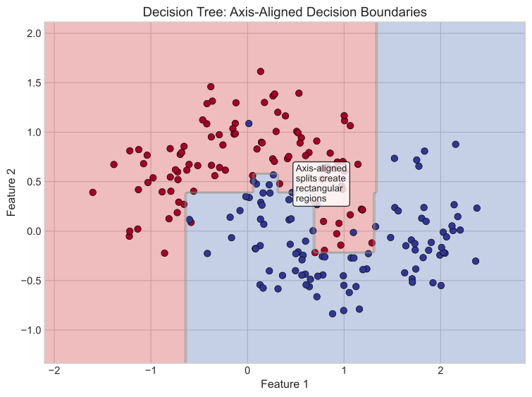
Decision trees create axis-aligned rectangular regions since each split divides along one feature at a time:

---

Splitting Criteria

For Classification

Criterion	Formula	Range (Binary)	Notes
Gini Impurity	$G(S)=1-\sum _i{p}_i^2$	0 to 0.5	Faster (no log)
Entropy	$H(S)=-\sum _i{p}_i{\log }_2(p_i)$	0 to 1.0	More balanced splits

Where $p_i$ is the proportion of class $i$ in set $S$.

Information Gain:

$$\text{IG}=H(\text{parent})-\sum _k\frac{|S_k|}{|S|}H(S_k)$$

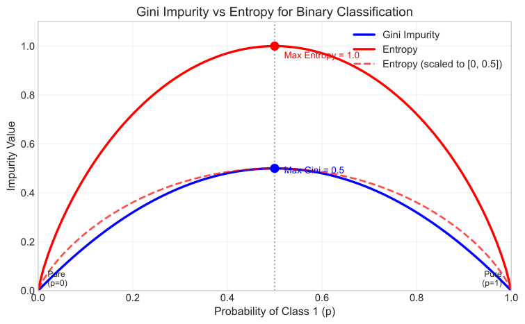
Gini vs Entropy: Very similar in practice (<2% accuracy difference). Gini is faster. Entropy tends to create more balanced trees.

For Regression

Criterion	Formula	Notes
MSE	$\frac{1}{n}\sum _i(y_i-\overline{y}{)}^2$	Standard choice
MAE	$\frac{1}{n}\sum_	y_i - \text{median}(y)

---

Split Selection Algorithm

def find_best_split(X, y, criterion='gini'):
    """Find the best feature and threshold to split on."""
    best_gain = -float('inf')
    best_feature, best_threshold = None, None
    current_impurity = compute_impurity(y, criterion)

    for feature_idx in range(X.shape[1]):
        for threshold in np.unique(X[:, feature_idx]):
            left_mask = X[:, feature_idx] <= threshold
            right_mask = ~left_mask

            if np.sum(left_mask) == 0 or np.sum(right_mask) == 0:
                continue

            # Weighted average of children impurities
            n_left, n_right = np.sum(left_mask), np.sum(right_mask)
            weighted_impurity = (
                (n_left / len(y)) * compute_impurity(y[left_mask], criterion) +
                (n_right / len(y)) * compute_impurity(y[right_mask], criterion)
            )

            gain = current_impurity - weighted_impurity
            if gain > best_gain:
                best_gain, best_feature, best_threshold = gain, feature_idx, threshold

    return best_feature, best_threshold, best_gain

---

Controlling Overfitting

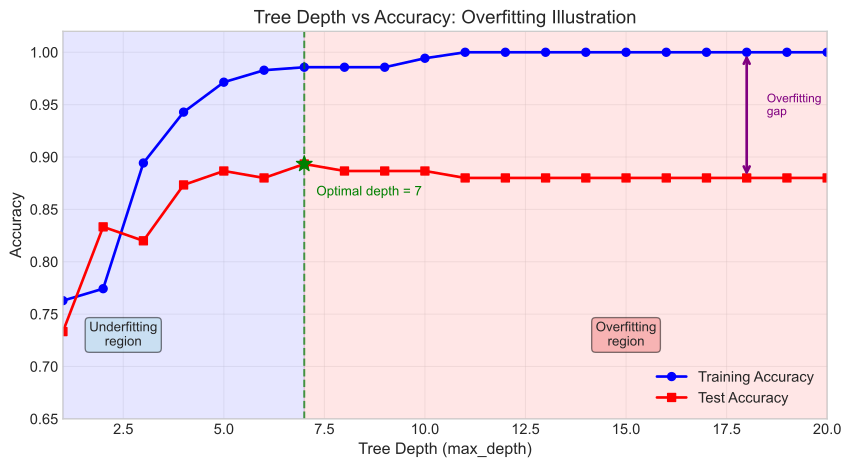
Decision trees are prone to overfitting. The graph below shows the classic bias-variance tradeoff:

Pre-Pruning (Early Stopping)

Parameter	Effect	Typical Range
max_depth	Limit tree depth	3-10
min_samples_split	Min samples to split a node	2-20
min_samples_leaf	Min samples in leaf	1-10
max_features	Features per split	sqrt(n), log2(n)
max_leaf_nodes	Maximum number of leaves	10-100

Post-Pruning (Cost-Complexity)

Grow full tree, then prune using:

$$\text{Cost}=\text{Error}+\alpha \times (\text{number of leaves})$$

• Reduced Error Pruning: Remove nodes if validation error doesn't increase
• Cost-Complexity Pruning: Cross-validate to find optimal $\alpha$

---

CART Algorithm

Classification And Regression Trees (CART):

• Binary splits only (left vs right)
• Gini for classification, MSE for regression
• Most common implementation (sklearn default)

Implementation

class DecisionTreeNode:
    def __init__(self, feature_idx=None, threshold=None,
                 left=None, right=None, value=None):
        self.feature_idx = feature_idx
        self.threshold = threshold
        self.left, self.right = left, right
        self.value = value  # Leaf prediction

    def is_leaf(self):
        return self.value is not None


class DecisionTree:
    def __init__(self, max_depth=None, min_samples_split=2):
        self.max_depth = max_depth
        self.min_samples_split = min_samples_split

    def fit(self, X, y):
        self.root = self._build_tree(X, y, depth=0)

    def _build_tree(self, X, y, depth):
        # Stopping conditions
        if (self.max_depth and depth >= self.max_depth) or \
           len(y) < self.min_samples_split or len(np.unique(y)) == 1:
            return DecisionTreeNode(value=np.argmax(np.bincount(y)))

        feat, thresh, gain = find_best_split(X, y)
        if gain <= 0:
            return DecisionTreeNode(value=np.argmax(np.bincount(y)))

        left_mask = X[:, feat] <= thresh
        return DecisionTreeNode(
            feature_idx=feat, threshold=thresh,
            left=self._build_tree(X[left_mask], y[left_mask], depth+1),
            right=self._build_tree(X[~left_mask], y[~left_mask], depth+1)
        )

    def predict(self, X):
        return np.array([self._traverse(x, self.root) for x in X])

    def _traverse(self, x, node):
        if node.is_leaf():
            return node.value
        if x[node.feature_idx] <= node.threshold:
            return self._traverse(x, node.left)
        return self._traverse(x, node.right)

---

Key Properties

Strengths	Weaknesses
Interpretable - visualize and explain decisions	Overfitting - deep trees memorize data
No scaling needed - invariant to feature scales	Instability - small data changes produce different trees
Handles mixed types - numerical and categorical	Axis-aligned splits - can't capture diagonal boundaries
Captures interactions - models feature relationships	Greedy - local optima may not be global
Fast prediction - $O(\log n)$ for balanced tree	Imbalanced data - biased toward majority class

---

Interview Questions

Q1: "How do you prevent overfitting in decision trees?"

Two approaches:

1. Pre-pruning - Stop growth early:

   • max_depth: Limit tree depth
   • min_samples_split/leaf: Require minimum samples

2. Post-pruning - Grow full tree, then remove nodes:

   • Cost-complexity pruning with $\alpha$ penalty
   • Cross-validate to find optimal complexity

Best practice: Use ensemble (Random Forest) which averages many trees to reduce variance.

Q2: "What's the difference between Gini and Entropy?"

Aspect	Gini	Entropy
Formula	$1-\sum p_i^2$	$-\sum p_i{\log }_2{p}_i$
Range (binary)	0 to 0.5	0 to 1.0
Speed	Faster (no log)	Slower
Splits	Similar	Slightly more balanced

Practical difference: <2% accuracy. Default to Gini (sklearn default).

Q3: "When would you use a decision tree vs. logistic regression?"

Use Decision Tree	Use Logistic Regression
Non-linear relationships	Linear relationship
Feature interactions ($X_1$ AND $X_2$)	Coefficient interpretation
Rules needed ("if income > 50K...")	Well-calibrated probabilities
Mixed feature types	High-dimensional data

Q4: "Why are decision trees unstable?"

Small changes in training data produce completely different trees because:

• Hierarchical structure: Different root split cascades everywhere
• Greedy optimization: Locally optimal splits
• Discrete splits: One point change can flip threshold

This variance hurts single trees but becomes diversity that helps ensembles (Random Forest, Bagging).

---

Comparison: Tree vs Linear

Aspect	Decision Tree	Linear Model
Decision boundary	Axis-aligned rectangles	Single hyperplane
Feature interactions	Captures naturally	Need explicit terms
Feature scaling	Not needed	Critical
Interpretability	Rules ("if X then Y")	Coefficients
Stability	Unstable (high variance)	Stable
Extrapolation	Constant prediction	Linear extrapolation

---

Quick Reference Card

DECISION TREE
---------------------------------------------
Algorithm: Recursively partition feature space
Splits:    Axis-aligned (one feature at a time)
Leaf:      Majority class (classification) or mean (regression)

SPLITTING CRITERIA
---------------------------------------------
Gini:    1 - Sum(p_i^2)     (faster)
Entropy: -Sum(p_i log2 p_i) (more balanced)
MSE:     Sum(y_i - y_bar)^2 (regression)

HYPERPARAMETERS
---------------------------------------------
max_depth:         Limit tree depth
min_samples_split: Min samples to split
min_samples_leaf:  Min samples in leaf
max_features:      Features per split

COMPLEXITY
---------------------------------------------
Training:   O(n * d * log n) average
Prediction: O(log n) to O(n) worst case
Space:      O(nodes)

USE WHEN
---------------------------------------------
+ Interpretable rules needed
+ Feature interactions important
+ Mixed feature types
- High-dimensional data (prefer ensemble)
- Need stable predictions