Transfer Learning Interview FAQ

Leverage pre-trained models for new tasks

Overview

Transfer learning reuses a model trained on one task as the starting point for a different but related task, dramatically reducing training time, data requirements, and computational costs.

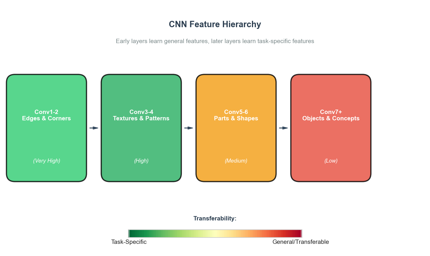
The key insight shown above: early layers learn general, transferable features while later layers become increasingly task-specific.

---

Interview Questions and Answers

Q1: What is transfer learning and when should you use it?

Answer:

Transfer learning uses a model trained on one task (the source task) as the starting point for a different task (the target task).

When to use:

• Limited labeled data - Small target dataset but related task has abundant data
• Computational constraints - Training from scratch is too expensive
• Similar domains - Source and target share underlying patterns
• State-of-the-art performance - Pre-trained models often outperform from-scratch training

When NOT to use:

• Very different domains - Features do not transfer well
• Abundant target data - Enough data to train from scratch
• Negative transfer risk - Source domain hurts target performance

---

Q2: What is the difference between feature extraction and fine-tuning?

Answer:

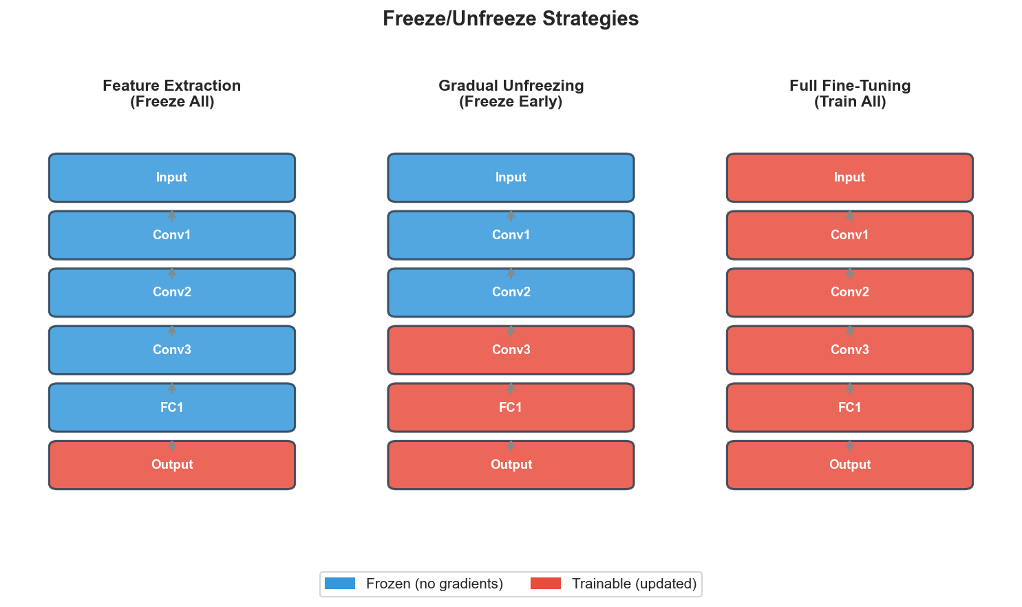
Aspect	Feature Extraction	Fine-Tuning
Layers trained	Classifier head only	Some/all layers
Training time	Fast	Slower
Data required	Very little	More
Overfitting risk	Lower	Higher
Performance ceiling	Lower	Higher

Workflow: Start with feature extraction baseline, then progressively fine-tune if needed.

---

Q3: Which layers should you freeze and why?

Answer:

Early layers learn general features (most transferable), later layers learn task-specific features (least transferable). Strategy depends on data size and domain similarity:

Scenario	Data	Domain Similarity	Strategy
A	Small	High	Freeze all, train classifier only
B	Small	Low	Freeze early, fine-tune later layers
C	Large	High	Fine-tune all with small LR
D	Large	Low	Fine-tune all, possibly larger LR

# Freeze all layers, then selectively unfreeze
for param in model.parameters():
    param.requires_grad = False
for param in model.layer4.parameters():  # Unfreeze last block
    param.requires_grad = True

---

Q4: What is domain adaptation?

Answer:

Domain adaptation addresses distribution shift between source and target domains.

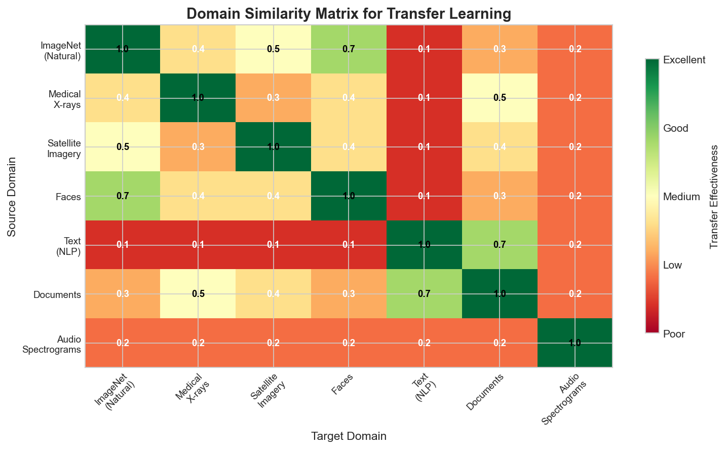
Types of domain shift: Covariate (input distributions differ), Prior (label distributions differ), Concept (input-output relationships differ)

Key techniques:

1. Feature alignment - MMD, DANN, CORAL
2. Instance weighting - Weight samples by similarity to target
3. Domain adversarial training - Feature extractor fools domain discriminator
4. Self-training - Pseudo-labels from target predictions

Examples: Sim-to-real robotics, cross-camera adaptation, cross-lingual NLP.

---

Q5: What are the major pre-trained models?

Answer:

Computer Vision:

Model	Parameters	Best For
ResNet-50	25M	Reliable baseline
EfficientNet	5-66M	Accuracy/efficiency tradeoff
ViT	86-632M	Large datasets
CLIP	400M	Zero-shot classification

NLP:

Model	Parameters	Best For
BERT	110-340M	Classification, NER, QA
GPT-2/3	117M-175B	Text generation
T5	60M-11B	Text-to-text tasks
LLaMA	7B-70B	Open-source NLP

Selection criteria: Task type, resource constraints, data availability, latency requirements, domain match.

---

Q6: What are effective fine-tuning strategies?

Answer:

Learning Rate:

• Use 10-100x smaller LR than from-scratch (1e-5 to 1e-4)
• Discriminative LR: Earlier layers get smaller LR, later layers get larger
• Warmup: Start very small, gradually increase (5-10% of training)

Unfreezing schedules:

Gradual: Epoch 1-2 head only -> Epoch 3-4 last block -> progressively unfreeze
All-at-once: Fine-tune all from start with very low LR + discriminative rates

Regularization:

• Dropout in new layers
• Lower weight decay than from-scratch
• Early stopping on validation loss
• Data augmentation (essential for small datasets)

Optimizers: AdamW for transformers, SGD with momentum for CNNs.

---

Q7: When does transfer learning fail (negative transfer)?

Answer:

Negative transfer occurs when pre-trained model hurts performance vs. from-scratch.

Causes:

• Domain mismatch (ImageNet to medical X-rays)
• Task mismatch (classification to dense prediction)
• Label space mismatch (fine-grained to coarse)
• Data quality differences

Detection:

• Compare against from-scratch baseline
• Monitor if loss decreases but accuracy stalls
• Visualize features (t-SNE)

Mitigation:

• Choose better source model closer to target domain
• Partial transfer (only early layers)
• Regularize toward pre-trained weights (L2-SP, EWC)
• Domain-adaptive pre-training

---

Q8: What is multi-task learning?

Answer:

Multi-task learning (MTL) trains one model on multiple related tasks simultaneously, allowing shared representations.

Aspect	Transfer Learning	Multi-Task Learning
Training	Sequential	Simultaneous
Goal	Improve target	Improve all tasks
Knowledge flow	One direction	Bidirectional

Architectures:

• Hard sharing: Shared hidden layers, task-specific heads
• Soft sharing: Separate models with similarity regularization

Benefits: Implicit data augmentation, regularization, efficiency.

Challenges: Task balancing, negative transfer between tasks, conflicting gradients.

Examples: BERT (MLM + NSP), T5 (unified text-to-text), multi-task CNNs.

---

Q9: Explain zero-shot and few-shot learning.

Answer:

Zero-Shot Learning:

• Classify samples from classes never seen during training
• Requires side information (attributes, text descriptions, embeddings)
• Example: CLIP matches images to text descriptions like "a photo of a zebra"

Few-Shot Learning:

• Learn new classes from K examples (typically K=1,5,10)
• K-shot N-way: K examples per class, N classes

Approaches:

1. Metric learning - Prototypical/Siamese networks learn similarity
2. Meta-learning - MAML learns to adapt quickly
3. Large model transfer - In-context learning (GPT-3)

Aspect	Zero-Shot	Few-Shot
Training examples	0	1-10 per class
Side info required	Yes	No
Accuracy	Lower	Higher

---

Q10: What is LoRA and parameter-efficient fine-tuning?

Answer:

PEFT updates only a small subset of parameters, keeping most frozen. Essential for large models where full fine-tuning is prohibitively expensive.

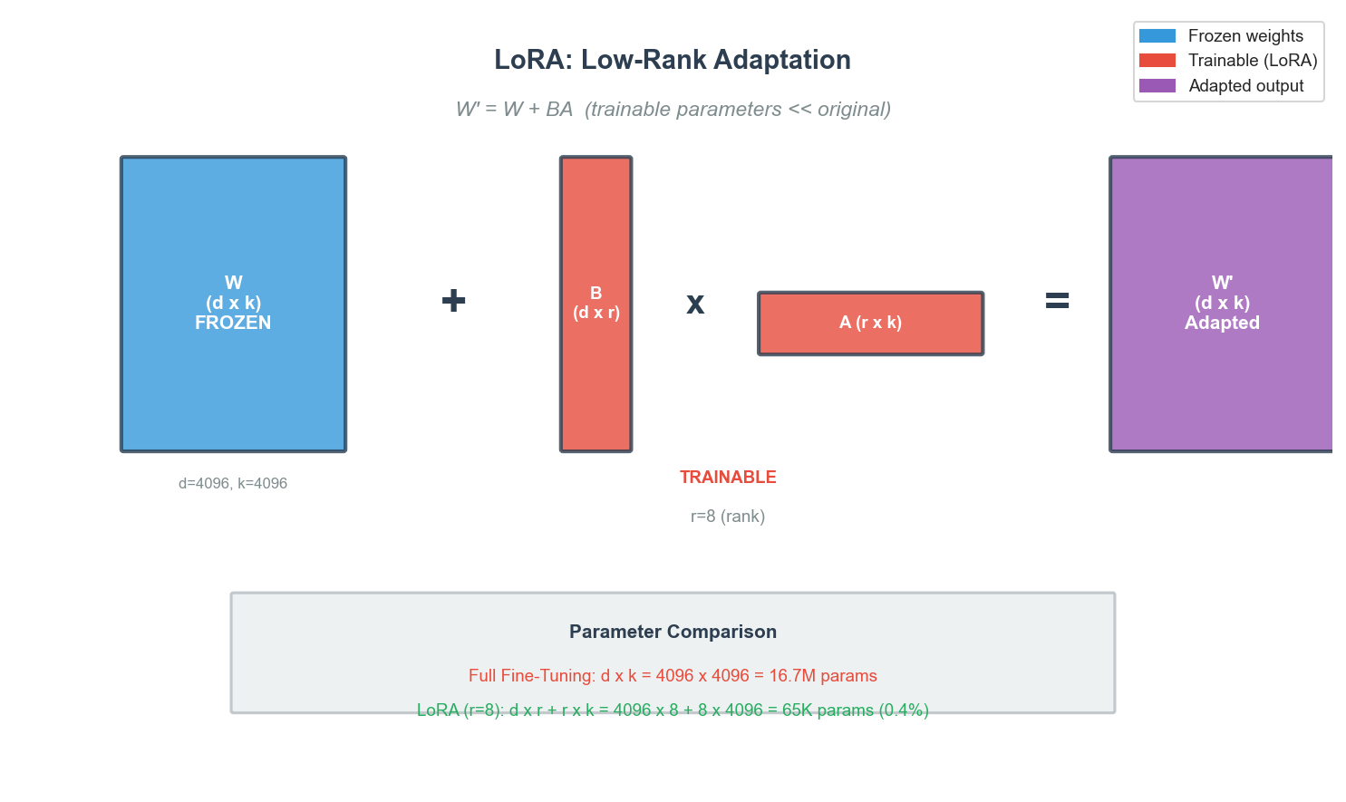
LoRA decomposes weight updates into low-rank matrices, reducing trainable parameters by 10,000x with no inference latency (merge after training).

PEFT Methods Comparison:

Method	Parameters Added
LoRA	0.1-1%
QLoRA	Even fewer (4-bit base)
Adapters	~3%
Prefix Tuning	~0.1%
Prompt Tuning	<0.01%

from peft import LoraConfig, get_peft_model

lora_config = LoraConfig(r=8, lora_alpha=32, target_modules=["q_proj", "v_proj"])
model = get_peft_model(base_model, lora_config)

---

Q11: How do you handle catastrophic forgetting?

Answer:

Catastrophic forgetting: Model forgets source knowledge when learning target task.

Mitigation strategies:

1. Regularization-based:

   • EWC: Penalize changing important weights (Fisher information)
   • L2-SP: L2 regularization toward pre-trained weights

2. Replay: Mix source data with target data during fine-tuning

3. Architecture-based: Adapters, progressive networks (add modules, freeze old)

4. Knowledge distillation: Use original model outputs as soft targets

def l2_sp_loss(model, original_params, lambda_sp=0.01):
    l2_sp = sum(((p - original_params[n]) ** 2).sum()
                for n, p in model.named_parameters() if n in original_params)
    return lambda_sp * l2_sp

---

Q12: How do you evaluate transfer learning effectiveness?

Answer:

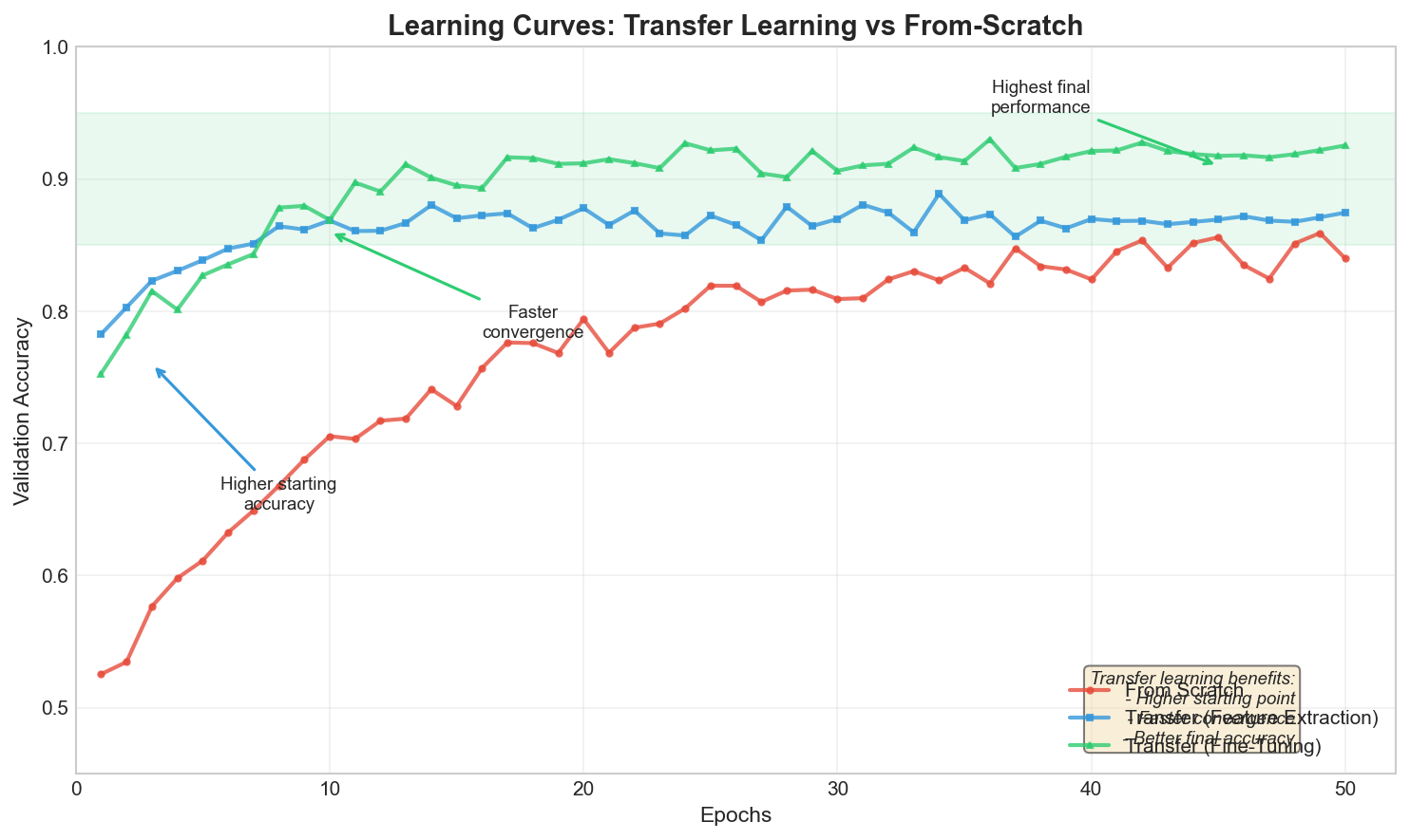
Key comparisons:

• Performance delta: Transfer vs. from-scratch accuracy
• Data efficiency: Target data needed to reach X% accuracy
• Time to convergence

Evaluation Protocol:

1. Train from-scratch baseline
2. Feature extraction baseline
3. Fine-tuning with various strategies
4. Compare all approaches

Best practices: Always include from-scratch baseline, report confidence intervals, test with varying target data amounts.

---

Q13: What is contrastive learning and self-supervised pre-training?

Answer:

Self-supervised learning creates pre-trained models without labels.

Contrastive Learning:

• Pull similar samples (positive pairs) closer
• Push dissimilar samples (negative pairs) apart

Key methods:

• SimCLR: Augmented views of same image are positives
• MoCo: Memory queue of negatives
• CLIP: Contrast images with text descriptions

InfoNCE Loss:

L = -log(exp(sim(z_i, z_j)/tau) / sum_k(exp(sim(z_i, z_k)/tau)))

Other self-supervised tasks: Masked language modeling (BERT), next token prediction (GPT), masked autoencoders (MAE).

---

Q14: How do you choose between transfer learning approaches?

Answer:

Decision framework:

Factor	Recommendation
Data < 1K	Feature extraction or heavy regularization
Data 1K-10K	Gradual unfreezing
Data > 10K	Full fine-tuning or from-scratch comparison
Same domain	Aggressive fine-tuning
Different domain	Careful layer selection, check negative transfer
Limited compute	Feature extraction or PEFT

Checklist:

1. Define target task and metrics
2. Assess target data quantity/quality
3. Identify closest pre-trained model
4. Start with feature extraction baseline
5. Try progressive fine-tuning
6. Compare against from-scratch
7. Check for negative transfer

---

Quick Reference Tables

Transfer Learning Methods

Method	Data Required	Compute	Best For
Feature Extraction	Very low	Low	Quick baseline, tiny datasets
Fine-tuning	Medium	Medium	Most scenarios
Domain Adaptation	Low-Medium	Medium	Distribution shift
PEFT (LoRA)	Low	Very low	Large models, limited resources

Learning Rate Guidelines

Approach	Typical LR
From scratch	1e-3 to 1e-2
Fine-tuning (full)	1e-5 to 1e-4
Fine-tuning (head only)	1e-3 to 1e-2
PEFT methods	1e-4 to 1e-3

---

Key Formulas

LoRA: W' = W + BA (r << d, k)

EWC: L = L_task + (lambda/2) * sum(F_i * (theta_i - theta*_i)^2)

InfoNCE: L = -log(exp(sim(z_i, z_j)/tau) / sum_k(exp(sim(z_i, z_k)/tau)))

---

Common Follow-ups

"How would you transfer from ImageNet to medical imaging?"

1. Start with feature extraction baseline
2. Fine-tune later layers with low LR
3. Consider domain-specific pre-trained models
4. Heavy data augmentation
5. Monitor for negative transfer

"When would you NOT use transfer learning?"

• Abundant target data
• Very different domains
• Real-time constraints prohibit large models
• Privacy concerns with pre-trained weights

"LoRA vs full fine-tuning?"

• LoRA: Limited GPU, multiple tasks, rapid iteration
• Full: Maximum performance needed, sufficient compute

---

Summary

1. Core concept: Reuse pre-trained knowledge for new tasks
2. Two approaches: Feature extraction (freeze all) vs fine-tuning (train some/all)
3. Layer selection: Early = general, later = task-specific
4. Domain adaptation: Handle distribution shift
5. PEFT: LoRA, adapters for efficient large model fine-tuning
6. Key risks: Negative transfer, catastrophic forgetting
7. Evaluation: Always compare against from-scratch baseline

---

Last updated: January 2026