Model Interpretability Interview FAQ

Explain black-box model predictions

---

Fundamentals of Interpretability

Q: Why is model interpretability important in machine learning?

A: Model interpretability is crucial for several interconnected reasons:

1. Trust and Adoption

• Stakeholders need to understand why a model makes certain predictions
• Users are more likely to adopt systems they can comprehend
• Domain experts can validate whether the model's reasoning aligns with reality

2. Debugging and Improvement

• Identify when models learn spurious correlations (e.g., detecting snow instead of huskies)
• Find data leakage issues where the model uses unintended features
• Understand failure modes and edge cases

3. Fairness and Bias Detection

• Reveal if protected attributes influence predictions inappropriately
• Ensure equitable treatment across demographic groups
• Support bias mitigation efforts

4. Regulatory Compliance

• Many industries require explainable decisions (healthcare, finance, legal)
• GDPR's "right to explanation" for automated decisions
• Model risk management in banking (SR 11-7)

5. Scientific Discovery

• Extract insights about underlying phenomena
• Generate hypotheses for further research
• Understand complex relationships in data

---

Q: What is the difference between intrinsic and post-hoc interpretability?

A: These represent two fundamentally different approaches to model explainability:

Intrinsic Interpretability: Models that are inherently interpretable by design.

Model Type	Interpretability Mechanism
Linear Regression	Coefficients show feature contributions
Decision Trees	Clear decision rules at each node
Rule Lists	Explicit if-then rules
GAMs	Additive contribution of each feature
Naive Bayes	Feature probability contributions

Advantages:

• Explanations are faithful to the actual model
• No additional computation needed
• Easier to audit and verify

Limitations:

• Often less accurate for complex problems
• May not capture non-linear interactions
• Limited expressiveness

Post-hoc Interpretability: Techniques applied after training to explain any model.

Technique	Type	Scope
SHAP	Model-agnostic	Local & Global
LIME	Model-agnostic	Local
Integrated Gradients	Gradient-based	Local
Attention Weights	Architecture-specific	Local
Partial Dependence	Model-agnostic	Global

Advantages:

• Works with any model (black-box compatible)
• Allows using high-performance complex models
• Flexible and adaptable

Limitations:

• Explanations may not perfectly reflect model behavior
• Additional computational cost
• May oversimplify complex interactions

---

Q: What is the difference between global and local explanations?

A: This distinction relates to the scope of the explanation:

Local Explanations: Explain individual predictions for specific instances.

Example: Why did the model predict THIS customer will churn?

Local Explanation:
- High monthly charges (+0.35 contribution)
- Short tenure (+0.28 contribution)
- No contract (-0.15 contribution)
- Final prediction: 78% churn probability

Use Cases:

• Individual decision justification
• Customer-facing explanations
• Debugging specific predictions
• Audit trails for compliance

Global Explanations: Explain overall model behavior across all predictions.

Example: What features matter most for churn prediction overall?

Global Explanation:
1. Contract type (importance: 0.32)
2. Monthly charges (importance: 0.24)
3. Tenure (importance: 0.21)
4. Internet service type (importance: 0.13)
5. Payment method (importance: 0.10)

Use Cases:

• Understanding model strategy
• Feature selection insights
• Communicating to stakeholders
• Model comparison

Bridging Local and Global:

# SHAP provides both through aggregation
import shap

# Local explanation for one instance
shap.waterfall_plot(shap_values[0])

# Global explanation by averaging absolute SHAP values
shap.summary_plot(shap_values, X)

---

SHAP (SHapley Additive exPlanations)

Q: What are SHAP values and how do they work?

A: SHAP values are a unified approach to explaining predictions based on game theory's Shapley values. SHAP distributes a prediction among features based on their contributions, treating features as "players" in a cooperative game.

Mathematical Foundation:

The Shapley value for feature i is:

φᵢ = Σ [|S|!(n-|S|-1)!/n!] × [f(S ∪ {i}) - f(S)]
     S⊆N\{i}

Where S is a subset of features not including i, n is the total number of features, and f(S) is the model prediction using only features in S.

Key Properties:

Property	Description	Formula
Efficiency	Values sum to prediction minus baseline	Σφᵢ = f(x) - E[f(x)]
Symmetry	Equal contribution = equal attribution	If f(S∪{i}) = f(S∪{j}) then φᵢ = φⱼ
Dummy	Zero contribution = zero attribution	If f(S∪{i}) = f(S) then φᵢ = 0
Additivity	Consistent across combined models	φᵢ(f+g) = φᵢ(f) + φᵢ(g)

Example Calculation:

import shap
import xgboost as xgb

# Train model and create explainer
model = xgb.XGBClassifier()
model.fit(X_train, y_train)
explainer = shap.TreeExplainer(model)
shap_values = explainer.shap_values(X_test)

# For a single prediction:
# Base value (average prediction): 0.3
# SHAP values: [0.15, -0.08, 0.12, 0.01]
# Prediction: 0.3 + 0.15 - 0.08 + 0.12 + 0.01 = 0.5

---

Q: What are the different SHAP explainer types and when should you use each?

A: SHAP provides several explainers optimized for different model types:

1. TreeExplainer

• For: Tree-based models (XGBoost, LightGBM, Random Forest, CatBoost)
• Speed: Very fast (polynomial time)
• Accuracy: Exact Shapley values

explainer = shap.TreeExplainer(xgb_model)
shap_values = explainer.shap_values(X)

2. DeepExplainer

• For: Deep learning models (TensorFlow, PyTorch)
• Speed: Fast (uses DeepLIFT approximation)
• Accuracy: Approximation based on reference distribution

explainer = shap.DeepExplainer(keras_model, X_background)
shap_values = explainer.shap_values(X_test)

3. GradientExplainer

• For: Neural networks
• Speed: Fast (gradient-based)
• Accuracy: Expected gradients approximation

explainer = shap.GradientExplainer(model, X_background)
shap_values = explainer.shap_values(X_test)

4. KernelExplainer

• For: Any model (model-agnostic)
• Speed: Slow (samples feature subsets)
• Accuracy: Approximation with convergence guarantees

explainer = shap.KernelExplainer(model.predict, X_background)
shap_values = explainer.shap_values(X_test, nsamples=1000)

5. LinearExplainer

• For: Linear models with correlated features
• Speed: Fast
• Accuracy: Exact for linear models

explainer = shap.LinearExplainer(linear_model, X_background)
shap_values = explainer.shap_values(X_test)

Selection Guide:

Model Type?
├── Tree-based → TreeExplainer
├── Deep Neural Network
│   ├── Need speed → GradientExplainer
│   └── Need accuracy → DeepExplainer
├── Linear Model → LinearExplainer
└── Any other → KernelExplainer

---

Q: How do you visualize and interpret SHAP values?

A: SHAP provides multiple visualization types for different analytical needs:

1. Summary Plot (Global) - Beeswarm

Shows feature importance with value distributions. Each dot is one prediction; color shows feature value (red=high, blue=low); horizontal position shows SHAP impact.

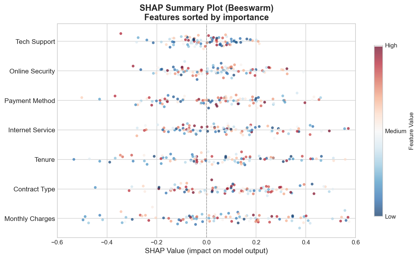
shap.summary_plot(shap_values, X)  # Beeswarm
shap.summary_plot(shap_values, X, plot_type="bar")  # Bar chart

2. Waterfall Plot (Local)

Shows how features push prediction from base value to final output for a single instance.

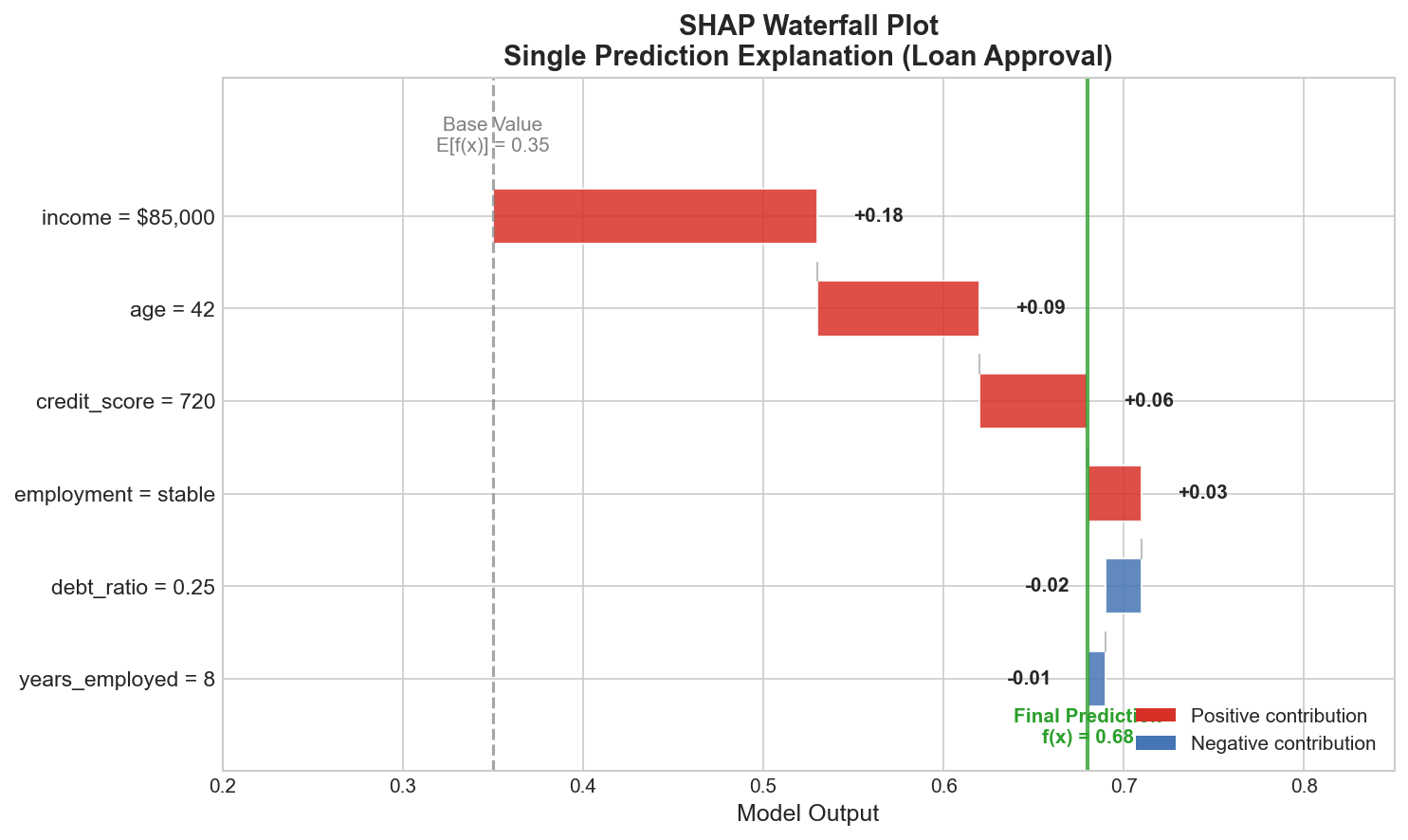
shap.waterfall_plot(shap_values[0])

3. Dependence Plot (Global)

Shows relationship between feature value and SHAP value, with interaction coloring revealing how other features affect the relationship.

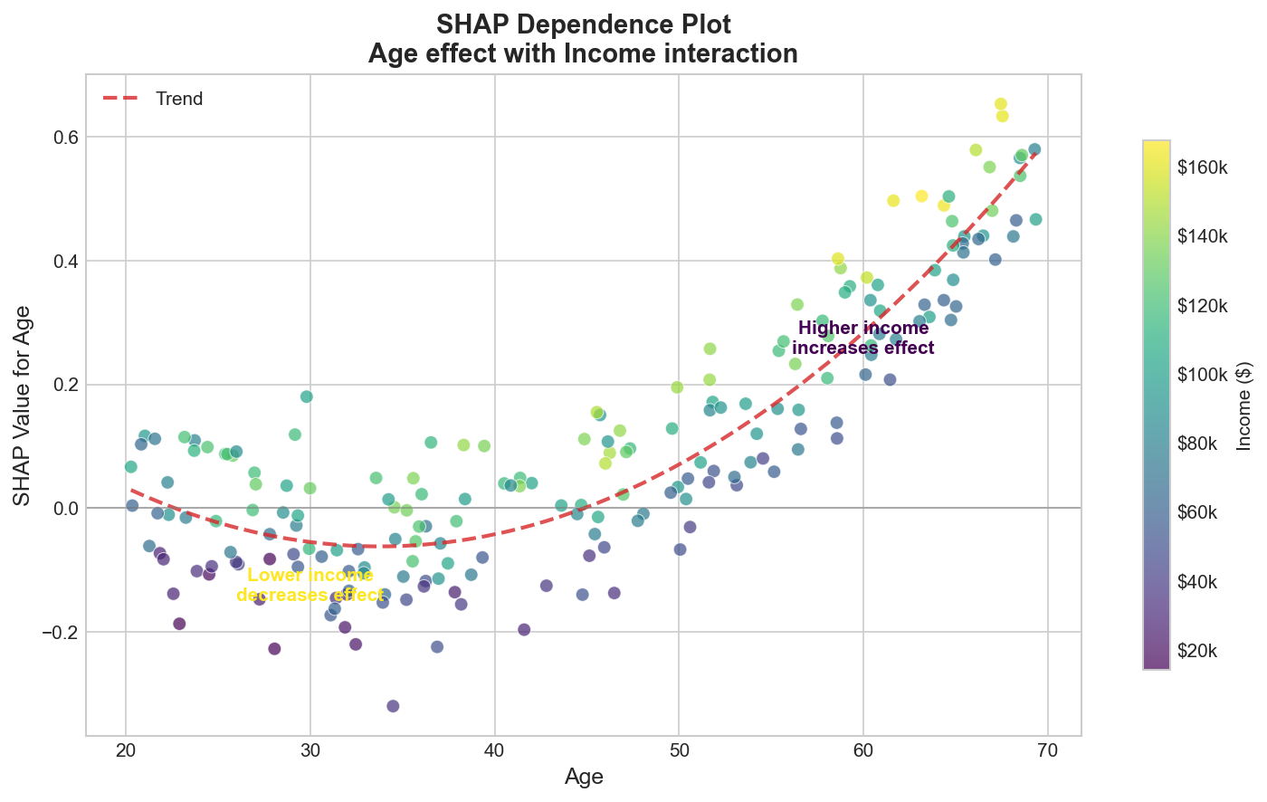
shap.dependence_plot("age", shap_values, X, interaction_index="income")

4. Interaction Values

interaction_values = explainer.shap_interaction_values(X)
shap.summary_plot(interaction_values, X)

---

LIME (Local Interpretable Model-agnostic Explanations)

Q: How does LIME work and what are its key principles?

A: LIME explains individual predictions by approximating the model locally with an interpretable model.

Algorithm Steps:

1. Select instance to explain
2. Generate perturbed samples around the instance
3. Get model predictions for perturbed samples
4. Weight samples by proximity to original instance
5. Fit interpretable model (e.g., linear regression) on weighted samples
6. Extract explanation from interpretable model

Mathematical Formulation:

ξ(x) = argmin L(f, g, πₓ) + Ω(g)
       g∈G

Where f is the original model, g is the interpretable model, πₓ is the proximity measure (kernel), and Ω(g) is the complexity penalty.

LIME Local Explanation Example:

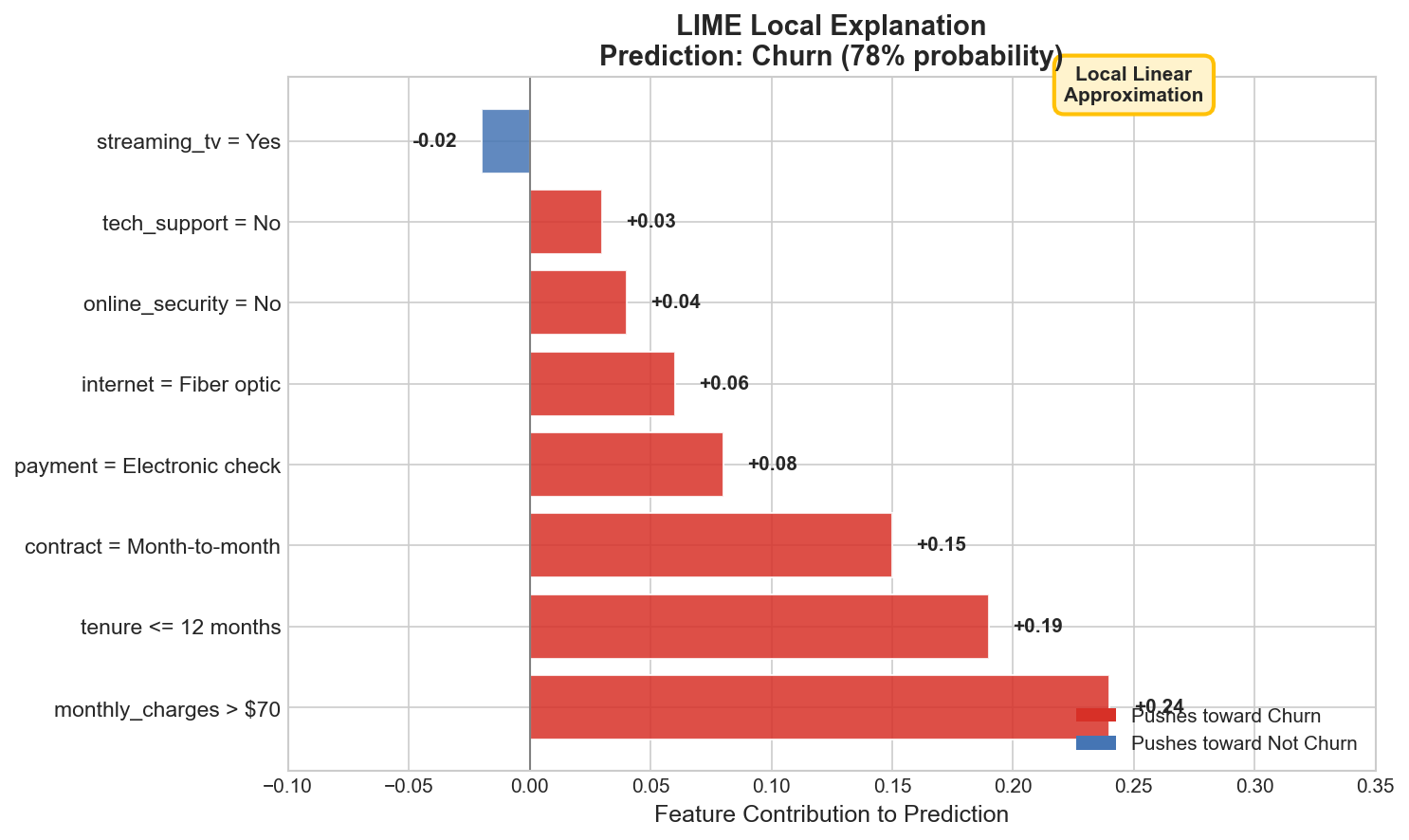
Implementation:

from lime import lime_tabular

explainer = lime_tabular.LimeTabularExplainer(
    training_data=X_train.values,
    feature_names=X_train.columns,
    class_names=['Not Churn', 'Churn'],
    mode='classification'
)

explanation = explainer.explain_instance(
    data_row=X_test.iloc[0].values,
    predict_fn=model.predict_proba,
    num_features=10,
    num_samples=5000
)
explanation.show_in_notebook()

---

Q: What are the differences between LIME and SHAP?

A: Both explain individual predictions but differ fundamentally:

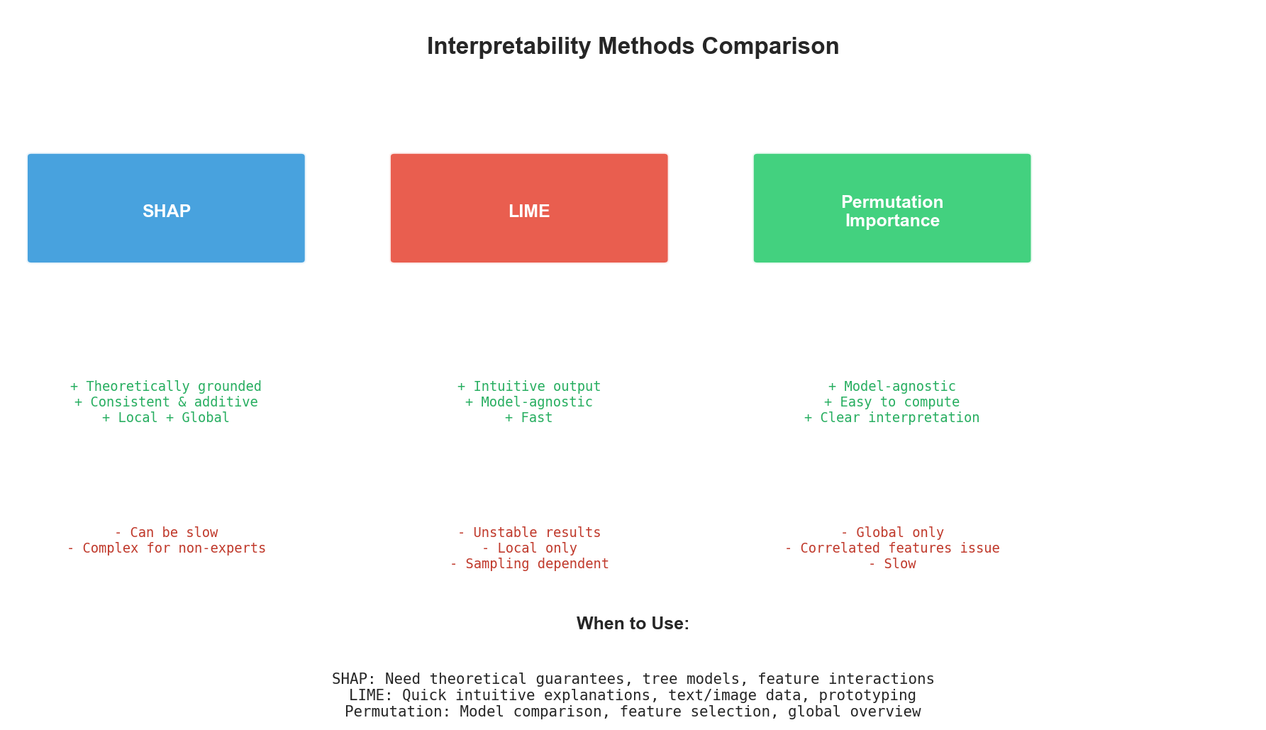
Aspect	LIME	SHAP
Theoretical Basis	Local linear approximation	Game-theoretic Shapley values
Consistency	Can vary between runs	Deterministic (exact methods)
Additivity	Not guaranteed	Guaranteed (values sum to prediction)
Computation	Sampling-based	Various (exact or approximation)
Scope	Primarily local	Local and global
Model Fidelity	Approximation in neighborhood	Exact for supported models

Consistency Comparison:

# LIME can produce different explanations for same instance
lime_exp1 = explainer.explain_instance(X[0], model.predict_proba)
lime_exp2 = explainer.explain_instance(X[0], model.predict_proba)
# May differ due to random sampling

# SHAP (TreeExplainer) is deterministic
shap_exp1 = explainer.shap_values(X[0:1])
shap_exp2 = explainer.shap_values(X[0:1])
# Always identical

When to Use Each:

Choose LIME	Choose SHAP
Quick, intuitive explanations	Need theoretical guarantees
Text or image data	Both local and global explanations
Human-friendly weights	Consistent, reproducible results
Unsupported model types	Tree-based models (very efficient)
	Feature interaction analysis

---

Q: How does LIME work for different data types (tabular, text, images)?

A: LIME adapts its perturbation strategy based on data type:

Tabular Data:

from lime.lime_tabular import LimeTabularExplainer

explainer = LimeTabularExplainer(
    X_train,
    feature_names=feature_names,
    categorical_features=categorical_indices,
    discretize_continuous=True
)

# Perturbation: Sample from training data distribution
# or discretize continuous features and flip values

Text Data:

from lime.lime_text import LimeTextExplainer

explainer = LimeTextExplainer(class_names=['Negative', 'Positive'])

def predict_fn(texts):
    # Convert texts to model input format
    return model.predict_proba(vectorizer.transform(texts))

explanation = explainer.explain_instance(
    text_instance="This movie was absolutely wonderful!",
    classifier_fn=predict_fn,
    num_features=10
)

# Perturbation: Remove words randomly
# Explanation: Which words contribute to prediction

Output:

Positive (0.92)
────────────────
wonderful  │ +0.35
absolutely │ +0.12
movie      │ +0.05
────────────────

Image Data:

from lime import lime_image
from skimage.segmentation import quickshift

explainer = lime_image.LimeImageExplainer()

explanation = explainer.explain_instance(
    image,
    classifier_fn=model.predict,
    top_labels=5,
    hide_color=0,
    num_samples=1000,
    segmentation_fn=quickshift
)

# Perturbation: Hide/show superpixels (segments)
# Explanation: Which regions contribute to prediction

---

Feature Importance Methods

Q: What are the different methods for calculating feature importance?

A: Several approaches exist, each with distinct properties:

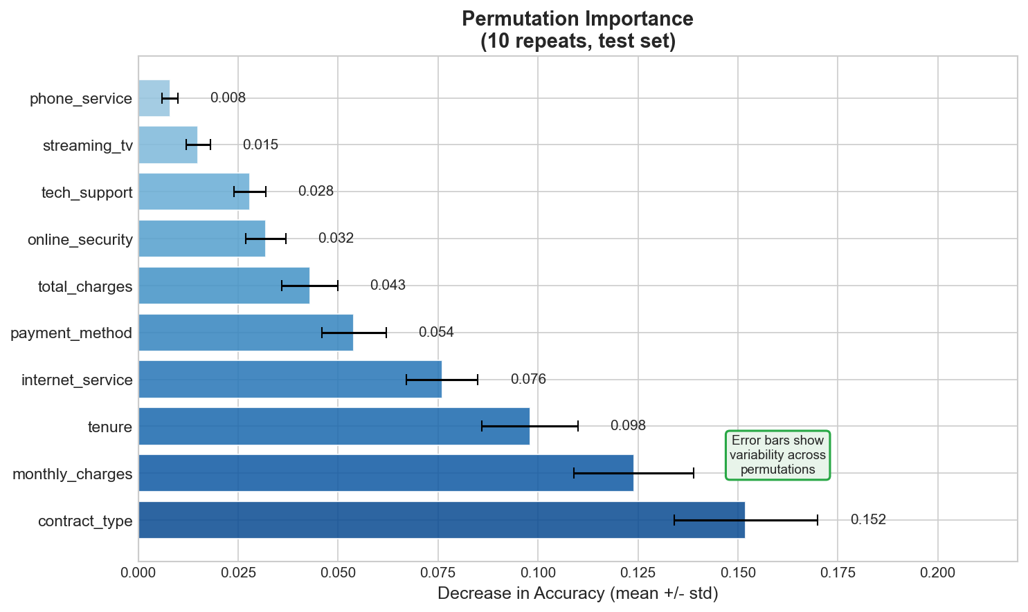
1. Permutation Importance

Measures importance by shuffling feature values and observing prediction degradation. Error bars show variability across multiple permutations.

from sklearn.inspection import permutation_importance

result = permutation_importance(
    model, X_test, y_test,
    n_repeats=10,
    random_state=42,
    scoring='accuracy'
)

for i in result.importances_mean.argsort()[::-1]:
    print(f"{feature_names[i]}: {result.importances_mean[i]:.4f} "
          f"(+/- {result.importances_std[i]:.4f})")

Pros: Model-agnostic, considers feature interactions | Cons: Slow, underestimates correlated features

2. Impurity-based Importance (Tree Models)

Based on total reduction in impurity from splits on each feature.

importances = model.feature_importances_  # Built into tree models

Pros: Fast, built-in | Cons: Biased toward high-cardinality features

3. SHAP-based Importance

Mean absolute SHAP values across all predictions.

shap_importance = np.abs(shap_values).mean(axis=0)
shap.summary_plot(shap_values, X, plot_type="bar")

Pros: Theoretically grounded, consistent | Cons: Computationally expensive for some models

4. Coefficient-based (Linear Models)

Absolute coefficient values with standardized features.

5. Drop-Column Importance

Train model without each feature and measure performance drop.

Pros: True feature contribution | Cons: Very slow (requires retraining)

---

Q: How do you handle correlated features in importance calculations?

A: Correlated features present challenges for importance methods:

The Problem:

Features: income, wealth (highly correlated, r=0.9)
True importance: Both equally important

Permutation importance might show:
- income: 0.15
- wealth: 0.05

Why? When income is shuffled, wealth still provides the signal.

Solutions:

1. Grouped Permutation Importance

def grouped_permutation_importance(model, X, y, feature_groups):
    """Permute correlated features together."""
    baseline = model.score(X, y)
    importances = {}

    for group_name, features in feature_groups.items():
        X_permuted = X.copy()
        for feat in features:
            X_permuted[feat] = np.random.permutation(X_permuted[feat])
        score = model.score(X_permuted, y)
        importances[group_name] = baseline - score

    return importances

# Example
groups = {
    'financial': ['income', 'wealth', 'assets'],
    'demographic': ['age', 'education']
}

2. Conditional Permutation

Permute feature while respecting conditional distribution given correlated features.

3. SHAP with Correlation Awareness

SHAP naturally handles correlations through its theoretical framework.

# Use interventional TreeExplainer
explainer = shap.TreeExplainer(
    model,
    feature_perturbation="interventional",
    data=X_background
)

4. Hierarchical Feature Importance

from scipy.cluster import hierarchy
from scipy.spatial.distance import squareform

# Cluster correlated features
corr_matrix = X.corr().abs()
distance_matrix = 1 - corr_matrix
linkage = hierarchy.ward(squareform(distance_matrix))

# Analyze importance at cluster level

---

Partial Dependence and Related Plots

Q: What are Partial Dependence Plots (PDPs) and ICE plots?

A: PDPs show the marginal effect of a feature on predictions (averaging out other features), while ICE plots show individual instance effects revealing heterogeneity.

Mathematical Definition:

PD(xₛ) = E_xc[f(xₛ, xc)] = (1/n) Σᵢ f(xₛ, xc⁽ⁱ⁾)

Where xₛ is the feature(s) of interest and xc are the other features (complement).

PDP with ICE Curves Visualization:

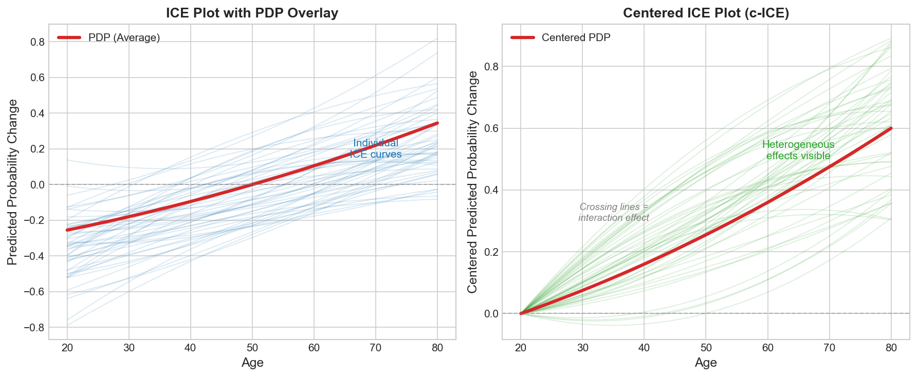
The left plot shows individual ICE curves (light blue lines) with the PDP average (red line). The right plot shows centered ICE (c-ICE) which makes it easier to compare curve shapes and detect interaction effects (crossing lines = interactions).

Implementation:

from sklearn.inspection import PartialDependenceDisplay

# ICE plot with PDP overlay
PartialDependenceDisplay.from_estimator(
    model, X, features=['age'],
    kind='both',  # Shows both ICE and PDP
    subsample=50
)

# Centered ICE
PartialDependenceDisplay.from_estimator(
    model, X, features=['age'],
    kind='individual',
    centered=True
)

When to Use:

PDP	ICE
Understand average effect	Check for heterogeneous effects
Present to stakeholders (simpler)	Detect interactions (crossing lines)
Feature independence assumed	Individual instance behavior

Limitations:

• PDPs assume feature independence (can show impossible combinations)
• Use ALE plots for correlated features

---

Q: What are Accumulated Local Effects (ALE) plots and when should you use them?

A: ALE plots address PDP limitations by using conditional distributions instead of marginal.

The Problem with PDPs:

If income and age are correlated:
- PDP might evaluate f(age=25, income=500k)
- This combination is unrealistic
- Leads to misleading interpretations

ALE Solution:

Instead of averaging over all other feature values, ALE:

1. Divides the feature into intervals
2. For each interval, calculates the average effect on predictions
3. Accumulates these local effects

Mathematical Definition:

ALE(x) = ∫ E[∂f/∂x | X=z] dz

Comparison:

Aspect	PDP	ALE
Handles correlation	No	Yes
Computation	Slower	Faster
Interpretation	Partial effect	Accumulated local effect
With interactions	Can mislead	More accurate

Implementation:

from alibi.explainers import ALE

ale = ALE(model.predict, feature_names=feature_names)
ale_explanation = ale.explain(X)

# Plot
import matplotlib.pyplot as plt
fig, ax = plt.subplots()
ax.plot(ale_explanation.ale_values[0])  # For first feature

When to Use ALE:

• Features are correlated
• Need faster computation
• Want more accurate effect estimates

When to Use PDP:

• Features are independent
• Need simpler interpretation
• Presenting to non-technical audience

---

Interpretability vs Accuracy Tradeoff

Q: How do you balance model interpretability with predictive accuracy?

A: This is a fundamental tension in ML system design:

The Traditional View:

        Accuracy
           ▲
           │     ○ Deep Neural Networks
           │   ○ Gradient Boosting
           │  ○ Random Forest
           │ ○ SVM
           │○ Logistic Regression
           ○ Decision Tree
           └─────────────────────▶ Interpretability

Modern Perspective:

The tradeoff is not always as stark:

1. GAMs with interactions can achieve near-GBDT performance
2. Attention mechanisms provide some interpretability in deep learning
3. Post-hoc methods (SHAP, LIME) explain complex models reasonably well

Decision Framework:

Start
  │
  ▼
Is high-stakes decision? ──Yes──▶ Prioritize interpretability
  │                                Use inherently interpretable models
  No                               Add extensive post-hoc analysis
  │
  ▼
Is accuracy critical? ──Yes──▶ Use best model + post-hoc explanations
  │                              Validate explanations carefully
  No
  │
  ▼
Use interpretable model
(GAM, Linear, Decision Tree)

Practical Strategies:

1. Interpretable First Approach

# Start with GAM
from interpret.glassbox import ExplainableBoostingClassifier

ebm = ExplainableBoostingClassifier()
ebm.fit(X_train, y_train)

# Check if accuracy is sufficient
ebm_score = ebm.score(X_test, y_test)

if ebm_score >= threshold:
    # Use interpretable model
    model = ebm
else:
    # Upgrade to complex model with explanations
    model = XGBClassifier()
    explainer = shap.TreeExplainer(model)

2. Explanation Fidelity Monitoring

def check_explanation_fidelity(model, explainer, X_sample):
    """Verify explanations are faithful to model."""
    shap_values = explainer.shap_values(X_sample)

    # SHAP values should sum to prediction difference
    base_value = explainer.expected_value
    predictions = model.predict(X_sample)

    reconstructed = base_value + shap_values.sum(axis=1)
    fidelity_error = np.abs(predictions - reconstructed).mean()

    return fidelity_error < 0.01  # Threshold for acceptable error

---

Q: What are Generalized Additive Models (GAMs) and why are they considered interpretable yet powerful?

A: GAMs extend linear models by allowing non-linear feature effects while maintaining additive structure.

Model Form:

g(E[y]) = β₀ + f₁(x₁) + f₂(x₂) + ... + fₚ(xₚ)

Where:

• g is a link function
• fᵢ are learned smooth functions (splines)
• No interactions between features (in basic form)

Why Interpretable:

• Each feature's effect can be visualized independently
• Effects are additive (easy to understand contributions)
• No hidden interactions

Why Powerful:

• Can capture non-linear relationships
• With pairwise interactions, can match gradient boosting
• Regularization prevents overfitting

Implementation:

from interpret.glassbox import ExplainableBoostingClassifier

# EBM = GAM with automatic interaction detection
ebm = ExplainableBoostingClassifier(
    interactions=10,  # Number of pairwise interactions
    max_bins=256,
    learning_rate=0.01
)
ebm.fit(X_train, y_train)

# Built-in visualization
from interpret import show
ebm_global = ebm.explain_global()
show(ebm_global)

Visualization Example:

Feature: age                    Feature: income
     ▲                               ▲
 0.3 │    ╭───╮                  0.2 │         ╭────
     │   ╱     ╲                     │     ╭───╯
 0.0 │──╯       ╲──              0.0 │─────╯
     │           ╲                   │
-0.2 │            ╲──           -0.2 │
     └─────────────────              └─────────────────
        20  40  60  80                  0   50k  100k

---

Regulatory Requirements

Q: What is the GDPR "right to explanation" and how does it impact ML systems?

A: GDPR Article 22 addresses automated decision-making:

Key Requirements:

1. Right Not to Be Subject to Automated Decisions

   • Individuals can opt out of purely automated decisions
   • Applies when decisions significantly affect them

2. Right to Meaningful Information

   • Must provide "meaningful information about the logic involved"
   • Include significance and envisaged consequences

3. Right to Human Review

   • Can request human intervention
   • Can express point of view and contest decision

What "Explanation" Means in Practice:

Minimum Requirements:
├── What data was used
├── How the decision was made (general logic)
├── What factors influenced the outcome
└── How to contest the decision

Best Practices:
├── Feature contributions for individual decisions
├── Counterfactual explanations
├── Uncertainty quantification
└── Clear documentation of model purpose

Compliance Implementation:

class ExplainableDecisionSystem:
    def __init__(self, model, explainer):
        self.model = model
        self.explainer = explainer

    def make_decision(self, applicant_data):
        # Make prediction
        prediction = self.model.predict(applicant_data)
        probability = self.model.predict_proba(applicant_data)

        # Generate explanation
        shap_values = self.explainer.shap_values(applicant_data)

        # Create decision record
        decision_record = {
            'decision': prediction,
            'confidence': probability,
            'timestamp': datetime.now(),
            'model_version': self.model.version,
            'features_used': list(applicant_data.columns),
            'top_factors': self._get_top_factors(shap_values),
            'explanation': self._generate_explanation(shap_values)
        }

        return decision_record

    def _generate_explanation(self, shap_values):
        """Generate human-readable explanation."""
        factors = []
        for i, (feat, val) in enumerate(zip(self.features, shap_values)):
            if abs(val) > 0.05:  # Significant contribution
                direction = "increased" if val > 0 else "decreased"
                factors.append(f"{feat} {direction} the likelihood")
        return "; ".join(factors)

---

Q: What are industry-specific regulations affecting model interpretability?

A: Different industries have specific requirements:

Financial Services (US):

Regulation	Requirement
SR 11-7 (Model Risk Management)	Document model methodology, assumptions, limitations
ECOA / Fair Lending	Adverse action notices with specific reasons
FCRA	Disclose key factors affecting credit decisions
CECL	Explainable loss forecasting models

Healthcare:

Regulation	Requirement
FDA (SaMD)	Clinical decision support must be transparent
HIPAA	Audit trails for automated decisions
Clinical Guidelines	Align with established medical knowledge

Insurance:

Regulation	Requirement
State Insurance Laws	Actuarial justification for pricing
Unfair Discrimination	No proxy discrimination
Rate Filing	Explain factors in premium calculation

Implementation for Adverse Action Notice:

def generate_adverse_action_notice(model, explainer, applicant_data, decision):
    """Generate compliant adverse action notice for credit decisions."""

    if decision == 'approved':
        return None

    # Get feature contributions
    shap_values = explainer.shap_values(applicant_data)

    # Map to reason codes (required by FCRA)
    reason_codes = {
        'credit_score': 'R01 - Credit score below threshold',
        'debt_to_income': 'R02 - Debt-to-income ratio too high',
        'employment_length': 'R03 - Insufficient employment history',
        'delinquencies': 'R04 - Recent delinquencies on record',
        'credit_utilization': 'R05 - High credit utilization'
    }

    # Get top 4 negative factors (FCRA requires up to 4)
    negative_factors = [
        (feat, val) for feat, val in zip(features, shap_values)
        if val < 0
    ]
    top_factors = sorted(negative_factors, key=lambda x: x[1])[:4]

    notice = {
        'decision': 'Application Declined',
        'principal_reasons': [
            reason_codes.get(feat, f'Factor: {feat}')
            for feat, _ in top_factors
        ],
        'credit_bureau_used': 'Experian',
        'contact_info': 'Call 1-800-XXX-XXXX for questions'
    }

    return notice

---

Counterfactual Explanations

Q: What are counterfactual explanations and how do they differ from feature attributions?

A: Counterfactual explanations describe how to change the input to get a different outcome.

Comparison:

Aspect	Feature Attribution	Counterfactual
Question	"Why this prediction?"	"What would change the prediction?"
Format	Feature importance scores	Actionable changes
Focus	Understanding	Action
Example	"Income contributed +0.3"	"Increase income by $10k to get approved"

Example:

Loan Application: DENIED

Feature Attribution (SHAP):
- Income: -0.25 (negative impact)
- Credit Score: -0.15 (negative impact)
- Debt Ratio: +0.05 (positive impact)
- Employment: +0.10 (positive impact)

Counterfactual Explanation:
To change outcome from DENIED to APPROVED:
Option 1: Increase income from $45k to $55k
Option 2: Improve credit score from 620 to 680
Option 3: Reduce debt ratio from 0.45 to 0.35

Implementation:

from dice_ml import Dice

# Create data interface
data = dice_ml.Data(
    dataframe=df,
    continuous_features=['income', 'age', 'credit_score'],
    outcome_name='approved'
)

# Create model interface
model = dice_ml.Model(model=sklearn_model, backend='sklearn')

# Create DiCE explainer
explainer = Dice(data, model)

# Generate counterfactuals
counterfactuals = explainer.generate_counterfactuals(
    query_instance=applicant_data,
    total_CFs=3,
    desired_class=1,  # Approved
    features_to_vary=['income', 'credit_score', 'debt_ratio']
)

counterfactuals.visualize_as_dataframe()

---

Q: What properties should good counterfactual explanations have?

A: Several desiderata for useful counterfactuals:

1. Validity The counterfactual should actually achieve the desired outcome.

def is_valid(original, counterfactual, model, target_class):
    return model.predict(counterfactual) == target_class

2. Proximity (Minimal Change) Changes should be as small as possible.

def proximity(original, counterfactual):
    # L1 distance (Manhattan)
    return np.abs(original - counterfactual).sum()

3. Sparsity Fewer features changed is better.

def sparsity(original, counterfactual, threshold=1e-4):
    return (np.abs(original - counterfactual) > threshold).sum()

4. Plausibility Counterfactual should be realistic (within data distribution).

def plausibility(counterfactual, data_distribution):
    # Could use density estimation
    return kde.score_samples(counterfactual.reshape(1, -1))[0]

5. Actionability Changes should be feasible for the user.

actionable_features = ['income', 'savings', 'debt']
immutable_features = ['age', 'race', 'gender']

# Only suggest changes to actionable features

6. Causally Consistent Respect causal relationships between features.

# If income increases, savings might also increase
# Counterfactual should reflect this

Complete Implementation:

def generate_optimal_counterfactual(
    original,
    model,
    target_class,
    actionable_features,
    data,
    max_iterations=1000
):
    """Generate counterfactual optimizing all desiderata."""

    cf = original.copy()
    best_cf = None
    best_score = float('inf')

    for _ in range(max_iterations):
        # Propose change
        feature = np.random.choice(actionable_features)
        change = np.random.normal(0, 0.1)

        cf_candidate = cf.copy()
        cf_candidate[feature] += change

        # Check validity
        if model.predict(cf_candidate.reshape(1, -1))[0] != target_class:
            continue

        # Calculate score (lower is better)
        score = (
            proximity(original, cf_candidate) +
            0.5 * sparsity(original, cf_candidate) -
            0.1 * plausibility(cf_candidate, data)
        )

        if score < best_score:
            best_score = score
            best_cf = cf_candidate.copy()

    return best_cf

---

Advanced Topics

Q: How do you explain predictions from deep learning models?

A: Deep learning requires specialized interpretability techniques:

1. Gradient-based Methods

# Vanilla Gradients
def vanilla_gradients(model, input_tensor, target_class):
    input_tensor.requires_grad = True
    output = model(input_tensor)
    output[0, target_class].backward()
    return input_tensor.grad

# Integrated Gradients
def integrated_gradients(model, input_tensor, baseline, target_class, steps=50):
    scaled_inputs = [baseline + (float(i)/steps) * (input_tensor - baseline)
                     for i in range(steps + 1)]
    gradients = [vanilla_gradients(model, inp, target_class) for inp in scaled_inputs]
    avg_gradients = torch.mean(torch.stack(gradients), dim=0)
    return (input_tensor - baseline) * avg_gradients

2. Attention-based Explanations

# For transformer models
def attention_explanation(model, input_ids):
    outputs = model(input_ids, output_attentions=True)
    attentions = outputs.attentions  # List of attention matrices

    # Average attention across heads and layers
    avg_attention = torch.mean(torch.stack(attentions), dim=(0, 1, 2))
    return avg_attention

3. Layer-wise Relevance Propagation (LRP)

Propagates relevance scores backward through the network.

4. Concept Activation Vectors (TCAV)

Tests if human-defined concepts influence model predictions.

# Example: Does the concept "stripes" influence zebra classification?
from tcav import TCAV

tcav = TCAV(model,
            concept_name='stripes',
            target_class='zebra',
            layer='conv5')

sensitivity = tcav.compute_tcav_score(test_images)
print(f"Zebra prediction is {sensitivity:.0%} sensitive to 'stripes' concept")

---

Q: How do you validate that explanations are faithful to the model?

A: Explanation fidelity is crucial for trustworthy interpretability:

1. Faithfulness Tests

def test_faithfulness(model, explainer, X, top_k=5):
    """Test if removing important features changes predictions."""

    faithfulness_scores = []

    for i, x in enumerate(X):
        # Get original prediction
        original_pred = model.predict_proba([x])[0, 1]

        # Get feature importance
        importance = explainer.explain(x)
        top_features = np.argsort(np.abs(importance))[-top_k:]

        # Mask top features
        x_masked = x.copy()
        x_masked[top_features] = 0  # Or use baseline values

        # Get new prediction
        masked_pred = model.predict_proba([x_masked])[0, 1]

        # Faithfulness = prediction change
        faithfulness_scores.append(abs(original_pred - masked_pred))

    return np.mean(faithfulness_scores)

2. Consistency Tests

def test_consistency(explainer, X, n_runs=10):
    """Test if explainer gives consistent results."""

    explanations = []
    for _ in range(n_runs):
        exp = explainer.explain(X[0])
        explanations.append(exp)

    # Calculate variance across runs
    variance = np.var(explanations, axis=0).mean()
    return variance < 0.01  # Should be very low

3. Sanity Checks

def model_parameter_randomization_test(model, explainer, X):
    """
    Explanations should change when model parameters are randomized.
    (Adebayo et al., 2018)
    """

    original_explanation = explainer.explain(X[0])

    # Randomize model parameters
    randomized_model = randomize_model_weights(model)
    randomized_explainer = create_explainer(randomized_model)

    random_explanation = randomized_explainer.explain(X[0])

    # Explanations should be different
    correlation = np.corrcoef(original_explanation, random_explanation)[0, 1]

    return correlation < 0.3  # Low correlation indicates valid explanation method

---

Q: What are the limitations and pitfalls of current interpretability methods?

A: Understanding limitations is crucial for responsible use:

1. LIME Instability

Problem: LIME results can vary significantly between runs

Mitigation:
- Increase num_samples
- Run multiple times and average
- Use deterministic random seed
- Consider SHAP for stability

2. SHAP Computational Cost

Problem: KernelSHAP is O(2^n) for exact computation

Mitigation:
- Use model-specific explainers (TreeSHAP)
- Sample-based approximation
- Background data sampling
- GPU acceleration

3. Feature Attribution Disagreement

Problem: Different methods give different explanations

Study results:
- Methods can rank features very differently
- No ground truth for real data
- Hard to know which is "correct"

Mitigation:
- Use multiple methods and look for consensus
- Validate with domain expertise
- Focus on top features (usually more consistent)

4. Explanation Manipulation

# Adversarial model that gives misleading explanations
# (Slack et al., 2020)

class BiasedExplainableClassifier:
    def __init__(self, biased_model, fair_model):
        self.biased_model = biased_model
        self.fair_model = fair_model

    def predict(self, X):
        # Use biased model for actual predictions
        return self.biased_model.predict(X)

    def predict_for_explanation(self, X):
        # Detect if being explained (OOD detection)
        if self._is_explanation_query(X):
            return self.fair_model.predict(X)
        return self.biased_model.predict(X)

5. Correlation vs Causation

Problem: Feature importance shows correlation, not causation

Example:
- "Ice cream sales" correlates with "drowning deaths"
- SHAP would show positive contribution
- Doesn't mean ice cream causes drowning

---

Quick Reference

Interpretability Method Selection Guide

What do you need to explain?
│
├── Individual Prediction
│   ├── Tree Model → TreeSHAP
│   ├── Neural Network → Integrated Gradients / DeepSHAP
│   ├── Any Model → KernelSHAP or LIME
│   └── Need Actionable Insight → Counterfactual
│
├── Overall Model Behavior
│   ├── Feature Importance → SHAP Summary / Permutation
│   ├── Feature Effects → PDP (independent features) / ALE (correlated)
│   └── Interactions → SHAP Interaction Values
│
└── Model Selection
    ├── High Stakes → Inherently Interpretable (GAM, Linear, Tree)
    └── Need Performance → Complex Model + Post-hoc Explanation

Common Interview Questions Summary

Question	Key Points
Why interpretability?	Trust, debugging, fairness, compliance, discovery
SHAP vs LIME	SHAP: consistent, additive; LIME: simple, unstable
Global vs Local	Global: overall behavior; Local: individual predictions
PDP limitations	Assumes independence, use ALE for correlated features
GDPR requirements	Meaningful information, right to contest, human review
Counterfactuals	Actionable, minimal, plausible changes
Deep learning	Gradients, attention, TCAV for concepts
Validation	Faithfulness, consistency, sanity checks

---

Key Takeaways

1. No Single Best Method: Different interpretability techniques suit different needs
2. Validate Explanations: Always verify faithfulness and consistency
3. Consider the Audience: Technical vs non-technical explanations differ
4. Regulatory Awareness: Know industry-specific requirements
5. Tradeoff Management: Balance interpretability with performance thoughtfully
6. Multiple Methods: Use complementary approaches for robust insights
7. Actionability: The best explanations lead to actionable insights
8. Limitations: Understand what explanations can and cannot tell you