Convolutional Neural Networks (CNNs)

The architecture for vision — leveraging spatial structure through convolutions

---

Why Not Fully Connected for Images?

A 224x224 RGB image has 150,528 values (50,176 pixels x 3 channels). A fully connected layer to 1000 hidden units needs 150 million weights — just for one layer.

Problems with FC for Images

Issue	Description
Too many parameters	Memory and computation explosion
No spatial structure	Treats adjacent pixels same as distant ones
Not translation invariant	Cat in corner vs center requires different weights
Overfitting	Huge parameter count with limited data

CNN Advantages

• Parameter sharing: Same filter applied everywhere
• Local connectivity: Each neuron sees only a small region
• Translation equivariance: Features detected regardless of position

---

The Convolution Operation

A convolution slides a small filter/kernel over the input, computing element-wise products and sums.

Mathematical Definition

For 2D input $I$ and filter $K$:

$$(I\ast K)[i,j]=\sum _m\sum _{n}I[i+m,j+n]\cdot K[m,n]$$

Example: 3x3 Filter on 5x5 Input

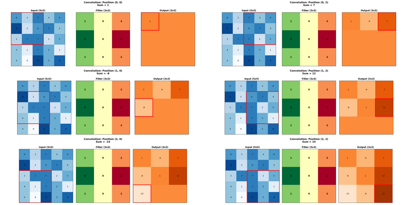
Input (5x5)              Filter (3x3)       Output (3x3)
┌────────────────┐       ┌───────┐          ┌──────────┐
│  1  2  3  4  5 │       │ 1 0 1 │          │ 35 40 45 │
│  6  7  8  9 10 │   *   │ 0 1 0 │    =     │ 60 65 70 │
│ 11 12 13 14 15 │       │ 1 0 1 │          │ 85 90 95 │
│ 16 17 18 19 20 │       └───────┘          └──────────┘
│ 21 22 23 24 25 │
└────────────────┘

Stride and Padding

Stride: How many pixels to move the filter each step

• Stride 1: Output slightly smaller than input
• Stride 2: Output half the size (used for downsampling)

Padding: Adding zeros around the input

• "Valid": No padding, output shrinks
• "Same": Pad to keep output same size as input

Output size formula:

$$\text{Output}=\lfloor \frac{\text{Input}+2\cdot \text{Padding}-\text{Filter}}{\text{Stride}}\rfloor +1$$

---

Key CNN Concepts

Multiple Filters = Multiple Feature Maps

Each filter detects one type of feature. A layer with 64 filters produces 64 feature maps.

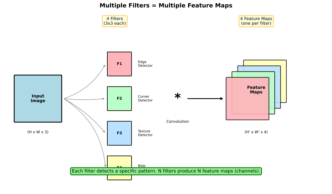
Channels/Depth

• Input: 3 channels (RGB)
• After conv layer with 64 filters: 64 channels
• Filter shape: (height, width, input_channels)
• Output shape: (height, width, num_filters)

Receptive Field

The receptive field is the input region that affects a particular output neuron.

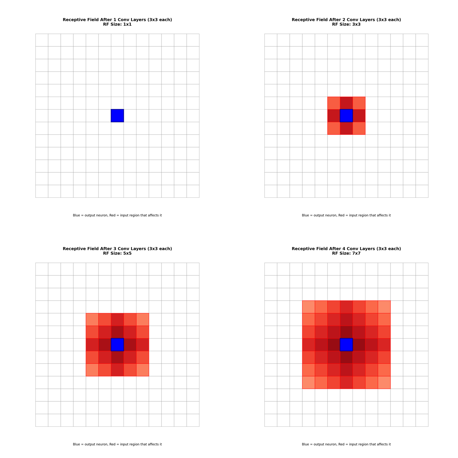
• Each conv layer increases receptive field by (kernel_size - 1)
• Deep networks have large receptive fields
• Important for capturing context (e.g., for segmentation)

---

Pooling Layers

Pooling reduces spatial dimensions while preserving important features.

Max Pooling vs Average Pooling

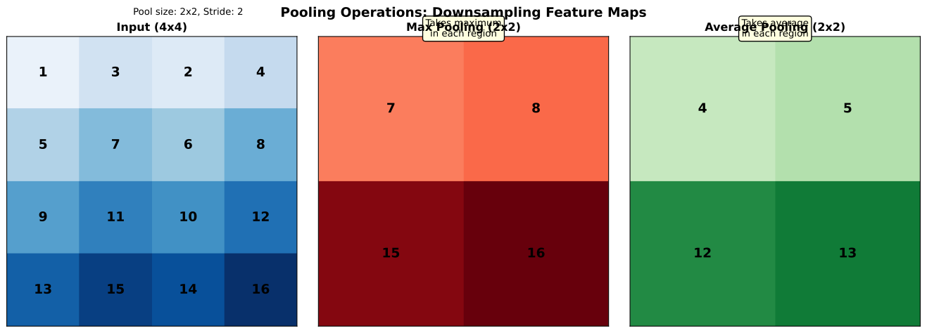
Input (4x4)              Max Pool (2x2)     Avg Pool (2x2)
┌───────────────┐        ┌───────┐          ┌───────┐
│ 1  3  2  4    │        │ 7  8  │          │ 4  5  │
│ 5  7  6  8    │   →    │ 15 16 │          │ 12 13 │
│ 9  11 10 12   │        └───────┘          └───────┘
│ 13 15 14 16   │
└───────────────┘

Max pooling: Takes maximum value — preserves strongest activation Average pooling: Takes mean — smoother downsampling

Why Pool?

1. Reduce computation: Smaller feature maps = faster processing
2. Translation invariance: Small shifts don't change max
3. Larger receptive field: Fewer pixels cover same input region

Modern Alternative: Strided Convolutions

Many modern architectures replace pooling with stride-2 convolutions:

• More learnable (filter weights vs fixed pooling)
• Smoother downsampling
• Used in ResNet, EfficientNet

---

Classic Architectures

LeNet (1998)

The original CNN for digit recognition:

Input → Conv → Pool → Conv → Pool → FC → FC → Output

AlexNet (2012)

Won ImageNet, sparked deep learning revolution:

• 5 conv layers, 3 FC layers
• ReLU activation (not sigmoid)
• Dropout for regularization
• GPU training

VGG (2014)

Simple principle: stack 3x3 convolutions

Two 3x3 convs have same receptive field as one 5x5
But fewer parameters and more non-linearity

ResNet (2015)

Introduced skip connections to train very deep networks.

---

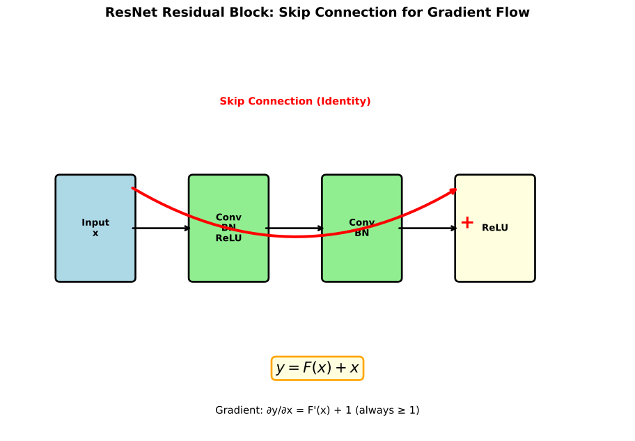
Skip Connections (Residual Blocks)

The key innovation of ResNet:

$$y=F(x)+x$$

Instead of learning $y=F(x)$, learn the residual $F(x)=y-x$.

Why Skip Connections Work

Gradient flow: Even if $F^{\prime }(x)\approx 0$, gradient can flow through the skip:

$$\frac{\partial y}{\partial x}=F^{\prime }(x)+1$$

Easier optimization: Learning $F(x)=0$ (identity) is easy — just set weights to zero.

Enables depth: ResNet-152 (152 layers) trains successfully; plain networks fail beyond ~20 layers.

Types of Skip Connections

Type	Formula	Used In
Residual	$y=F(x)+x$	ResNet
Dense	$y=F([x_1,x_2,\dots ,x_n])$	DenseNet
Highway	$y=F(x)\cdot T(x)+x\cdot (1-T(x))$	Highway Networks

---

Modern Convolution Variants

1x1 Convolutions

A 1x1 conv is a channel mixer — combines channels without spatial processing:

# 256 channels → 64 channels (dimension reduction)
nn.Conv2d(256, 64, kernel_size=1)

Uses:

• Reduce channels (bottleneck in ResNet)
• Increase channels cheaply
• Add non-linearity between large convolutions

Depthwise Separable Convolutions

Split convolution into:

1. Depthwise: One filter per input channel (spatial only)
2. Pointwise: 1x1 conv to mix channels

Efficiency: Much fewer parameters than standard conv Used in: MobileNet, EfficientNet

Dilated/Atrous Convolutions

Insert gaps in the filter to increase receptive field without more parameters:

Standard 3x3:     Dilated 3x3 (rate=2):
[X X X]           [X . X . X]
[X X X]           [. . . . .]
[X X X]           [X . X . X]

Used in: Semantic segmentation (DeepLab)

---

CNN for Different Tasks

Task	Output	Architecture
Classification	Single label	CNN → Global Pool → FC → Softmax
Detection	Boxes + labels	CNN → Region proposals → FC
Segmentation	Pixel labels	Encoder → Decoder (U-Net)

Transfer Learning

Pre-trained CNNs (on ImageNet) transfer well:

1. Load pre-trained weights
2. Replace final FC layer for new task
3. Fine-tune with lower learning rate

---

Interview Questions

Q1: "Why do we use convolutions instead of fully connected layers for images?"

Three key reasons:

1. Parameter efficiency: A 3x3 conv has 9 parameters per channel pair. FC connecting 224x224 to 1000 units needs 150M parameters. Convolutions share weights across spatial positions.

2. Spatial locality: Images have local structure — nearby pixels are related. Convolutions capture this with local receptive fields. FC treats all pixels equally, ignoring spatial relationships.

3. Translation equivariance: The same filter applied everywhere detects features regardless of position. A cat detector works whether the cat is in the corner or center. FC would need separate weights for each position.

Result: CNNs need fewer parameters, generalize better, and are computationally tractable for high-resolution images.

Q2: "Explain skip connections and why they help."

Skip connections add the input directly to the output:

$$y=F(x)+x$$

Why they help:

1. Gradient highway: The gradient flows directly through the skip: $\frac{\partial y}{\partial x}=F^{\prime }(x)+1$. Even if $F^{\prime }(x)\approx 0$ (vanishing gradient), the +1 ensures gradient reaches early layers.

2. Easier optimization: The network only needs to learn the residual $F(x)=y-x$. If the identity is optimal, just learn $F(x)=0$ (set weights to zero). This is easier than learning the full transformation.

3. Enables depth: Without skip connections, plain networks beyond ~20 layers degrade (not just overfit — training error increases). With skips, ResNet-152 trains successfully.

Key insight: Skip connections change the problem from "learn y" to "learn how y differs from x."

Q3: "What is the receptive field and why does it matter?"

Receptive field: The region of input that influences a particular output neuron.

How it grows:

• Each conv layer increases by (kernel_size - 1)
• Each pooling/stride-2 layer doubles it
• Dilated convolutions increase it without more parameters

Why it matters:

1. Context: For classification, the receptive field should cover the whole object. For segmentation, it should capture context around each pixel.

2. Architecture design: Too small = can't see enough context. Too large = may be wasteful.

3. Depth requirement: A network needs enough layers for its receptive field to cover relevant input regions.

Example: A 7-layer network with 3x3 convs has receptive field of 15x15. This may be too small for 224x224 ImageNet images — need deeper networks or dilated convolutions.

---

Key Takeaways

1. Convolutions exploit spatial structure through local connectivity and weight sharing.

2. Pooling/striding reduces spatial dimensions while increasing receptive field.

3. Skip connections enable very deep networks by providing gradient highways.

4. 1x1 convolutions mix channels efficiently — crucial in modern architectures.

5. Receptive field determines context — must be large enough to capture relevant input regions.

6. Modern CNNs use depthwise separable convs, efficient blocks, and transfer learning.