Generative Adversarial Networks (GANs)

Learning through competition — generator vs discriminator in a minimax game

---

The GAN Framework

GANs train two networks that compete against each other:

• Generator $G$: Creates fake data from random noise
• Discriminator $D$: Distinguishes real data from fake

The Minimax Game

$$\underset{G}{min}\underset{D}{max}V(D,G)={\mathbb{E}}_{x\sim p_{data}}[\log D(x)]+{\mathbb{E}}_{z\sim p_z}[\log (1-D(G(z)))]$$

• $D$ tries to maximize: Correctly classify real as real ($D(x)\to 1$) and fake as fake ($D(G(z))\to 0$)
• $G$ tries to minimize: Fool $D$ into thinking fake is real ($D(G(z))\to 1$)

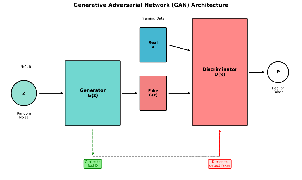
Training Flow

1. Sample real data x from dataset
2. Sample noise z from prior (e.g., Gaussian)
3. Generate fake data: x_fake = G(z)
4. Train D to distinguish x from x_fake
5. Train G to fool D (make D(G(z)) → 1)
6. Repeat

---

Training Dynamics

Alternating Optimization

for epoch in range(epochs):
    # Train Discriminator
    real_loss = BCE(D(x_real), ones)
    fake_loss = BCE(D(G(z)), zeros)
    d_loss = real_loss + fake_loss
    d_loss.backward()
    optimizer_D.step()

    # Train Generator
    g_loss = BCE(D(G(z)), ones)  # Want D to think fake is real
    g_loss.backward()
    optimizer_G.step()

Non-Saturating Generator Loss

The original $G$ loss $\log (1-D(G(z)))$ has vanishing gradients when $D$ is strong.

Fix: Use $-\log (D(G(z)))$ instead:

• Same optimum
• Stronger gradients early in training

---

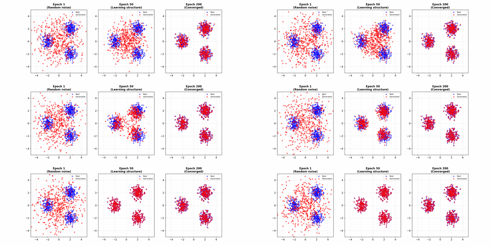
Mode Collapse

The most notorious GAN problem: generator produces limited variety.

What Happens

Instead of learning the full data distribution, the generator finds a few "safe" outputs that consistently fool the discriminator.

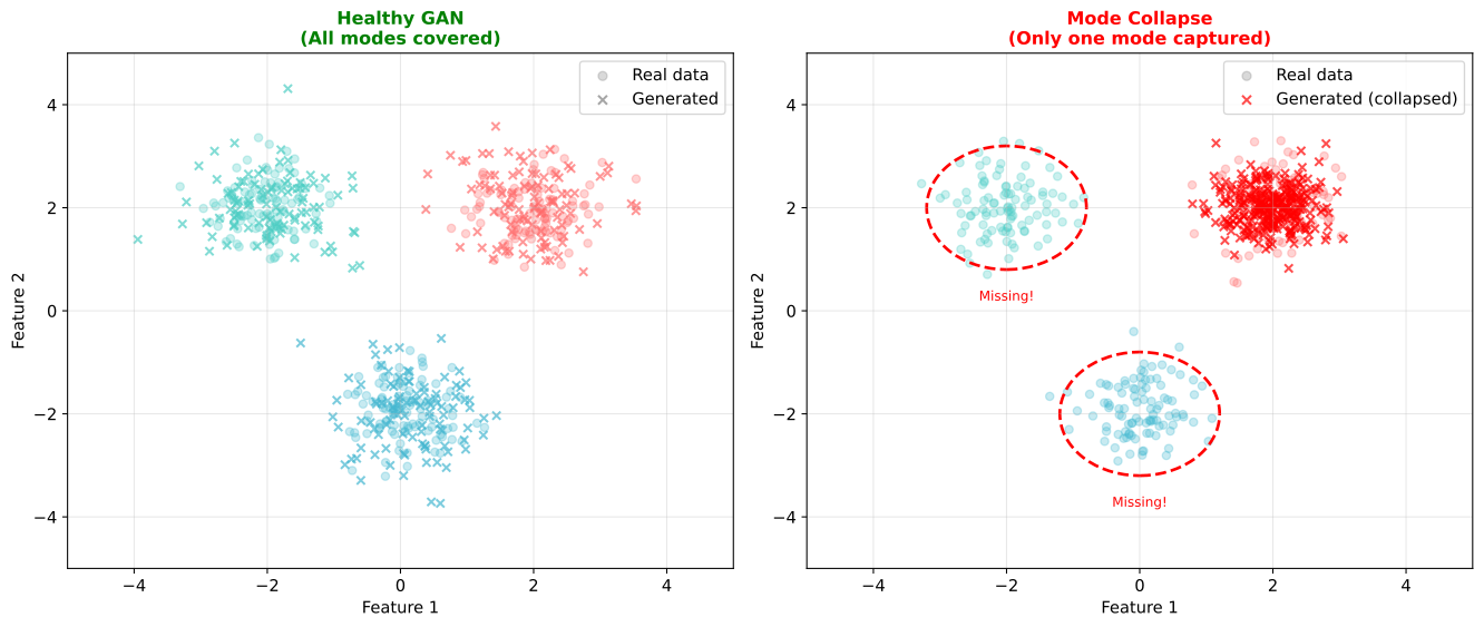
Example: Training on MNIST, generator only produces 3s and 7s, ignoring other digits.

Why It Happens

• Discriminator gives similar feedback for all outputs
• Generator finds local optimum that works
• No incentive to explore other modes

Solutions

Method	How It Helps
WGAN	Wasserstein distance provides better gradients
Minibatch discrimination	D sees batches, detects lack of diversity
Unrolled GANs	G anticipates D's future updates
Feature matching	G matches feature statistics, not just fools D
Progressive growing	Start small, gradually increase resolution

---

Training Instability

GANs are notoriously hard to train.

Problems

1. Vanishing gradients: When D is too strong, G gets no useful gradient
2. Oscillation: D and G chase each other, never converging
3. Sensitivity: Hyperparameters matter enormously
4. No good stopping criterion: Hard to tell when training is "done"

Practical Tips

Tip	Rationale
Use spectral normalization	Stabilizes D training
Train D more than G	Keep D slightly ahead
Use label smoothing	Prevent D from being overconfident
Add noise to D inputs	Regularization
Use progressive growing	Easier optimization
Monitor FID during training	Detect divergence

---

Wasserstein GAN (WGAN)

WGAN addresses training instability by changing the loss function.

The Problem with JS Divergence

Original GAN minimizes Jensen-Shannon divergence. When distributions don't overlap:

• JS divergence saturates
• Gradients vanish
• G can't improve

Wasserstein Distance (Earth Mover's Distance)

$$W(P_r,P_g)=\underset{\gamma \in \mathrm{\Pi }(P_r,P_g)}{inf}{\mathbb{E}}_{(x,y)\sim \gamma }[||x-y||]$$

Intuitively: minimum "work" to transform one distribution into another.

Key property: Provides meaningful gradients even when distributions don't overlap.

WGAN Training

Replace discriminator with critic (no sigmoid, outputs real number):

$$L={\mathbb{E}}_{x\sim p_{data}}[D(x)]-{\mathbb{E}}_{z\sim p_z}[D(G(z))]$$

Critic must be 1-Lipschitz (bounded gradient). Enforced by:

• Weight clipping (original WGAN): Clip weights to [-c, c]
• Gradient penalty (WGAN-GP): $\lambda \mathbb{E}[(||{\mathrm{\nabla }}_{x}D(x)|{|}_2-1{)}^2]$

Why WGAN Works

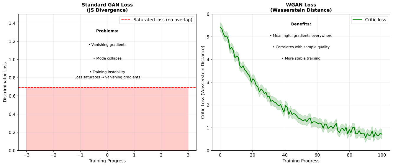
Aspect	Vanilla GAN	WGAN
Loss metric	JS divergence	Wasserstein distance
Gradient behavior	Can vanish	Always meaningful
Training stability	Sensitive	More stable
Mode collapse	Common	Reduced

---

GAN Variants

DCGAN (Deep Convolutional GAN)

Architecture guidelines for stable training:

• Use strided convolutions (no pooling)
• Use BatchNorm in G and D
• Use ReLU in G, LeakyReLU in D
• No fully connected layers (except G input, D output)

StyleGAN

A landmark GAN architecture for high-quality face generation:

• Mapping network transforms noise
• Style injection at each layer
• Progressive growing
• Explicit control over styles

Conditional GAN (cGAN)

Generate specific classes by conditioning on labels:

G(z, class_label) → image of that class
D(x, class_label) → real/fake for that class

Pix2Pix / CycleGAN

Image-to-image translation:

• Pix2Pix: Paired training data (sketch → photo)
• CycleGAN: Unpaired data (horse → zebra)

---

Evaluation Metrics

Evaluating GANs is notoriously difficult.

Inception Score (IS)

$$IS=\exp ({\mathbb{E}}_x[D_{KL}(p(y|x)||p(y))])$$

• Higher is better
• Measures quality (confident classifications) and diversity
• Limitation: Doesn't compare to real data distribution

Frechet Inception Distance (FID)

$$FID=||{\mu }_r-{\mu }_g|{|}^2+\text{Tr}({\mathrm{\Sigma }}_r+{\mathrm{\Sigma }}_g-2({\mathrm{\Sigma }}_r{\mathrm{\Sigma }}_g{)}^{1/2})$$

• Lower is better
• Compares feature distributions of real vs generated
• More reliable than IS
• Most commonly reported metric

Human Evaluation

For specific applications, nothing beats human judgment:

• A/B testing: Which looks more real?
• Task-specific metrics (e.g., face landmark accuracy)

---

Interview Questions

Q1: "Explain mode collapse and how to address it."

Mode collapse: The generator produces limited variety, ignoring some modes (clusters) of the real data distribution.

Example: Training on MNIST, generator only outputs certain digits, not all 10.

Why it happens:

• Generator finds outputs that consistently fool discriminator
• No explicit diversity objective
• Local optimum that's hard to escape

Solutions:

1. WGAN with gradient penalty: Wasserstein loss provides better gradients, less prone to collapse
2. Minibatch discrimination: Discriminator sees batches, can detect lack of diversity
3. Feature matching: Generator matches feature statistics, not just discriminator output
4. Unrolled GANs: Generator anticipates discriminator's future updates
5. Multiple generators: Each generates different modes

Detection: Monitor sample diversity during training, use FID which captures mode coverage.

Q2: "Why is WGAN more stable than vanilla GAN?"

Vanilla GAN uses JS divergence, which has problems:

• When real and generated distributions don't overlap, JS divergence is constant (maxed out)
• Gradients vanish, generator can't improve
• This happens early in training when G is bad

WGAN uses Wasserstein distance (Earth Mover's Distance):

$$W(P_r,P_g)=\underset{\gamma }{inf}{\mathbb{E}}_{(x,y)\sim \gamma }[||x-y||]$$

Key properties:

• Continuous and differentiable almost everywhere
• Provides meaningful gradients even when distributions don't overlap
• Correlates with sample quality (can monitor during training)

Implementation:

• Replace sigmoid discriminator with linear critic
• Enforce 1-Lipschitz constraint via gradient penalty

Result: More stable training, reduced mode collapse, better correlation between loss and quality.

Q3: "How do you evaluate GAN quality?"

FID (Frechet Inception Distance) — most common:

• Extract features from real and generated images using pretrained network
• Compute mean and covariance of feature distributions
• FID measures distance between these Gaussians
• Lower is better, typically in range 1-100+
• Good because it compares to real data distribution

Inception Score (IS):

• Measures classification confidence and diversity
• Higher is better
• Limitation: Doesn't compare to real data

Human evaluation:

• Gold standard for perceptual quality
• A/B tests, preference studies
• Expensive and slow

Task-specific metrics:

• Face generation: Landmark accuracy, identity preservation
• Super-resolution: PSNR, SSIM

What to report: FID is standard. Also report sample images for qualitative assessment.

---

Key Takeaways

1. GANs are a minimax game — generator creates fakes, discriminator detects them.

2. Mode collapse is the main failure mode — generator produces limited variety.

3. WGAN stabilizes training by using Wasserstein distance with gradient penalty.

4. FID is the standard metric — lower is better, measures distribution similarity.

5. Training is sensitive — requires careful hyperparameter tuning, architecture choices.

6. Many variants exist for different tasks: StyleGAN for faces, Pix2Pix for image translation, conditional GANs for controlled generation.