Actor-Critic Methods

Best of both worlds — combining policy gradients with value function estimation

---

The Motivation: Why Combine Approaches?

Reinforcement learning has two fundamental paradigms for learning optimal behavior:

Value-Based Methods (e.g., Q-learning, DQN):

• Learn a value function $Q(s,a)$ or $V(s)$
• Derive policy implicitly: $\pi (s)=\arg \underset{a}{max}Q(s,a)$
• Low variance but biased estimates
• Struggle with continuous action spaces

Policy Gradient Methods (e.g., REINFORCE):

• Learn a parameterized policy ${\pi }_{\theta }(a|s)$ directly
• Use Monte Carlo returns for gradient estimation
• High variance but unbiased
• Handle continuous actions naturally

Actor-Critic methods elegantly combine both approaches, using a value function to reduce variance while maintaining the flexibility of policy gradients.

---

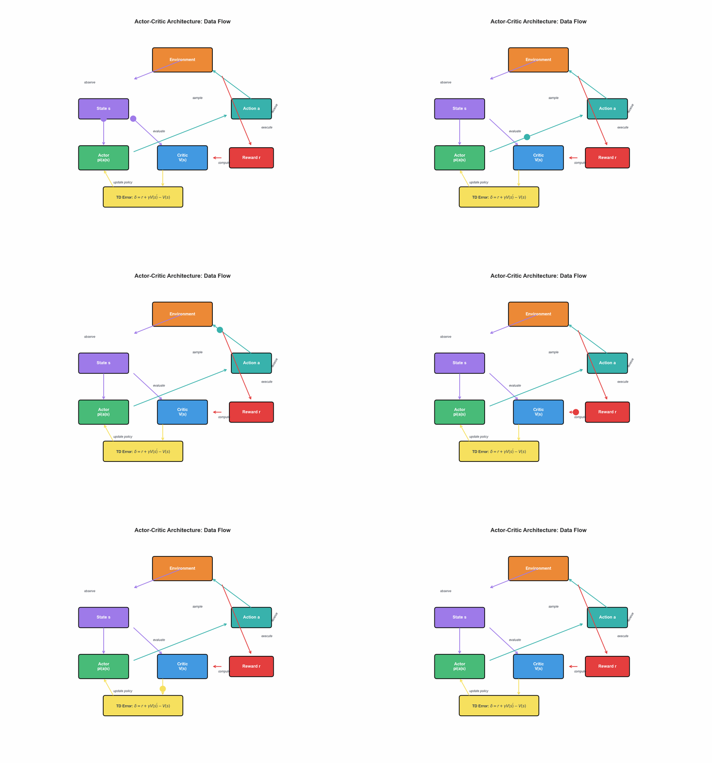
The Actor-Critic Framework

Two Networks, One Goal

The architecture consists of two components trained simultaneously:

Component	Role	Output	Objective
Actor	Policy network	${\pi }_{\theta }(a|s)$	Maximize expected return
Critic	Value network	$V_{\varphi }(s)$ or $Q_{\varphi }(s,a)$	Minimize TD error

The actor decides what action to take, while the critic evaluates how good that action was. The critic's feedback guides the actor's learning, reducing the variance inherent in pure policy gradient methods.

The Learning Loop

At each timestep $t$:

1. Actor samples action $a_t\sim {\pi }_{\theta }(\cdot |s_t)$
2. Environment returns reward $r_t$ and next state $s_{t+1}$
3. Critic computes TD error: ${\delta }_t=r_t+\gamma V_{\varphi }(s_{t+1})-V_{\varphi }(s_t)$
4. Update Critic: minimize ${\delta }_t^2$
5. Update Actor: use ${\delta }_t$ as advantage estimate

---

TD Error as Advantage Estimate

From Returns to Advantages

In vanilla REINFORCE, the policy gradient is:

$${\mathrm{\nabla }}_{\theta }J(\theta )=\mathbb{E}[\sum _t{\mathrm{\nabla }}_{\theta }\log {\pi }_{\theta }(a_t|s_t)\cdot G_t]$$

where $G_t=\sum _{k=0}^{\mathrm{\infty }}{\gamma }^k{r}_{t+k}$ is the Monte Carlo return. This has high variance because $G_t$ depends on the entire future trajectory.

Key insight: We can subtract a baseline $b(s_t)$ without introducing bias:

$${\mathrm{\nabla }}_{\theta }J(\theta )=\mathbb{E}[\sum _t{\mathrm{\nabla }}_{\theta }\log {\pi }_{\theta }(a_t|s_t)\cdot (G_t-b(s_t))]$$

The optimal baseline is the value function $V(s_t)$, giving us the advantage:

$$A(s_t,a_t)=G_t-V(s_t)$$

The advantage tells us: "How much better was this action compared to the average action from this state?"

One-Step TD Error Approximation

Computing the full return $G_t$ still requires waiting for episode completion. The TD error provides a one-step approximation:

$${\delta }_t=r_t+\gamma V(s_{t+1})-V(s_t)$$

This is an unbiased estimate of the advantage under certain conditions:

$$\mathbb{E}[{\delta }_t|s_t,a_t]=\mathbb{E}[r_t+\gamma V(s_{t+1})|s_t,a_t]-V(s_t)=Q(s_t,a_t)-V(s_t)=A(s_t,a_t)$$

The TD error enables online learning without waiting for episode termination.

---

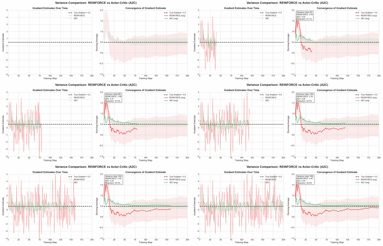
Why Actor-Critic Reduces Variance

The Variance Problem in REINFORCE

Consider the REINFORCE gradient with return $G_t$:

Writing $X={\mathrm{\nabla }}_{\theta }\log \pi$ and $Y=G_t$, the variance of the product depends on the spread of both factors. For independent $X$ and $Y$ the exact decomposition is:

$$\text{Var}[XY]=\text{Var}[X]\text{Var}[Y]+\text{Var}[X](\mathbb{E}[Y]{)}^2+(\mathbb{E}[X]{)}^2\text{Var}[Y]$$

In practice the score function $X$ and the return $Y$ are not independent, so this is only illustrative — but it makes the key point clear: variance grows with both the magnitude of the return $G_t$ and the spread of the score-function term.

The variance of $G_t$ is large because it accumulates randomness from:

• Stochastic policy sampling
• Environment transitions
• Rewards across many timesteps

How the Critic Helps

By subtracting the value baseline:

$$\text{Var}[{\delta }_t]=\text{Var}[r_t+\gamma V(s_{t+1})-V(s_t)]$$

This has much lower variance because:

1. Single-step: Only one reward and transition, not entire trajectory
2. Centering: Subtracting $V(s_t)$ centers the signal around zero
3. Bootstrapping: $V(s_{t+1})$ provides a stable target

---

Advantage Actor-Critic (A2C)

Synchronous Training

A2C is the synchronous variant of A3C (described below). It runs multiple environments in parallel, collects experiences, and performs a single synchronized update.

Algorithm:

Initialize actor parameters theta, critic parameters phi
for each iteration:
    Collect trajectories from N parallel environments for T steps
    Compute advantages: A_t = sum_{k=0}^{n-1} gamma^k r_{t+k} + gamma^n V(s_{t+n}) - V(s_t)

    Actor loss: L_actor = -mean(log pi_theta(a|s) * A)
    Critic loss: L_critic = mean((V_phi(s) - V_target)^2)
    Entropy bonus: H = -mean(sum pi log pi)

    Total loss: L = L_actor + c1 * L_critic - c2 * H
    Update theta, phi using gradient descent

n-Step Returns

Rather than using single-step TD, A2C typically uses n-step returns for lower bias:

$$G_t^{(n)}=r_t+\gamma r_{t+1}+\cdots +{\gamma }^{n-1}{r}_{t+n-1}+{\gamma }^{n}V(s_{t+n})$$

The n-step advantage becomes:

$$A_t^{(n)}=G_t^{(n)}-V(s_t)$$

n	Bias	Variance	Use Case
1	High	Low	Fast updates, stable environments
5	Medium	Medium	General purpose (common default)
$\mathrm{\infty }$	Zero	High	Monte Carlo (episodic tasks)

Entropy Regularization

To encourage exploration, A2C adds an entropy bonus to the loss:

$$H({\pi }_{\theta })=-\sum _a{\pi }_{\theta }(a|s)\log {\pi }_{\theta }(a|s)$$

This prevents the policy from becoming too deterministic too early, promoting exploration of the action space.

---

Asynchronous Advantage Actor-Critic (A3C)

Parallel Workers Architecture

A3C runs multiple worker threads asynchronously, each interacting with its own environment instance. Workers compute gradients locally and update a shared global network.

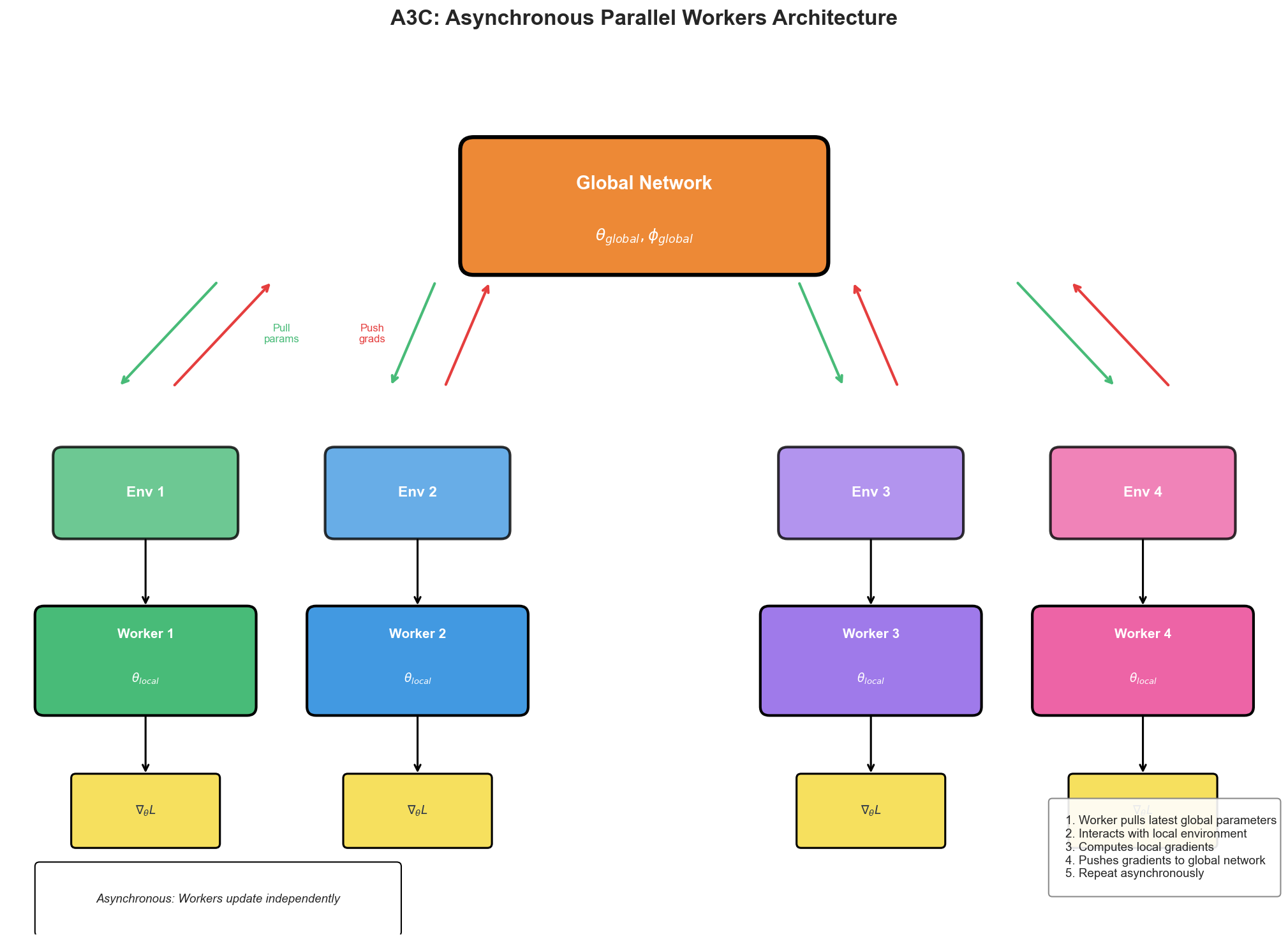
Why Asynchronous?

1. Decorrelated updates: Different workers experience different states, reducing correlation in gradient updates
2. Efficient CPU utilization: No GPU required; workers run on CPU cores
3. Implicit exploration: Asynchronous updates create natural variation in policies
4. No replay buffer: Online learning without the memory overhead of experience replay

A3C vs A2C Trade-offs

Aspect	A3C (Asynchronous)	A2C (Synchronous)
Updates	Asynchronous, may conflict	Batched, consistent
Hardware	CPU-efficient	GPU-friendly
Stability	Can be unstable	More stable
Implementation	Complex threading	Simpler batching
Modern preference	Less common	Preferred

In practice, A2C is now preferred because modern hardware (GPUs, TPUs) benefits more from batched synchronous updates, and the stability improvements outweigh the theoretical benefits of asynchrony.

---

Architecture Considerations

Shared vs Separate Networks

Shared Architecture (common for simple tasks):

State s --> [Shared Layers] --> Actor Head (policy)
                            --> Critic Head (value)

Separate Architecture (better for complex tasks):

State s --> [Actor Network] --> Policy
State s --> [Critic Network] --> Value

Shared architectures have fewer parameters and can transfer learned representations, but may suffer from interference between policy and value learning.

Network Design Guidelines

Consideration	Recommendation
Activation	ReLU or Tanh for hidden layers
Output (Actor)	Softmax for discrete, Gaussian parameters for continuous
Output (Critic)	Linear (unbounded value)
Initialization	Orthogonal init, smaller weights for output layers
Learning rate	Often different for actor (lower) vs critic (higher)

Handling Continuous Actions

For continuous action spaces, the actor outputs parameters of a Gaussian distribution:

$${\pi }_{\theta }(a|s)=\mathcal{N}({\mu }_{\theta }(s),{\sigma }_{\theta }(s{)}^2)$$

The network outputs $\mu$ and $\log \sigma$ (log for numerical stability), and actions are sampled via the reparameterization trick:

$$a={\mu }_{\theta }(s)+{\sigma }_{\theta }(s)\cdot ϵ,ϵ\sim \mathcal{N}(0,1)$$

---

Quick Reference

+------------------------------------------------------------------+
|                    ACTOR-CRITIC CHEAT SHEET                       |
+------------------------------------------------------------------+

CORE COMPONENTS:
  Actor:  pi_theta(a|s)    - Policy network, selects actions
  Critic: V_phi(s)         - Value network, evaluates states

TD ERROR (Advantage Estimate):
  delta_t = r_t + gamma * V(s_{t+1}) - V(s_t)

POLICY GRADIENT WITH BASELINE:
  grad_theta J = E[grad log pi_theta(a|s) * A(s,a)]

A2C LOSS FUNCTION:
  L = L_actor + c1 * L_critic - c2 * H(pi)
  where:
    L_actor  = -E[log pi * A]          (maximize advantage)
    L_critic = E[(V - V_target)^2]     (minimize TD error)
    H(pi)    = -E[sum pi log pi]       (entropy bonus)

N-STEP RETURNS:
  G_t^(n) = r_t + gamma*r_{t+1} + ... + gamma^{n-1}*r_{t+n-1} + gamma^n*V(s_{t+n})
  A_t^(n) = G_t^(n) - V(s_t)

VARIANCE REDUCTION:
  REINFORCE: Uses G_t (full return) -> High variance
  Actor-Critic: Uses delta_t (TD error) -> Lower variance

KEY HYPERPARAMETERS:
  gamma:       Discount factor (0.99 typical)
  n-steps:     Bootstrapping horizon (5 typical)
  c1:          Critic loss coefficient (0.5 typical)
  c2:          Entropy coefficient (0.01 typical)
  lr_actor:    Actor learning rate (often 1e-4)
  lr_critic:   Critic learning rate (often 1e-3)

+------------------------------------------------------------------+

---

Interview Questions

Question 1: Why does actor-critic have lower variance than REINFORCE?

Sample Answer:

REINFORCE uses the full Monte Carlo return $G_t=\sum _{k=0}^{\mathrm{\infty }}{\gamma }^k{r}_{t+k}$ as the learning signal. This accumulates variance from every future timestep, including stochastic transitions and rewards across the entire trajectory.

Actor-Critic replaces this with the TD error ${\delta }_t=r_t+\gamma V(s_{t+1})-V(s_t)$, which reduces variance in three ways:

1. Single-step signal: Only one transition contributes randomness, not the entire future trajectory

2. Baseline subtraction: By subtracting $V(s_t)$, we center the signal around zero. When the advantage is near zero (action was average), the gradient update is small, reducing noisy updates

3. Bootstrapping from learned value: The critic provides a learned estimate $V(s_{t+1})$ that summarizes expected future returns, replacing the noisy sampled return with a smoother function

The trade-off is introducing bias since $V(s)$ is an approximation, but the variance reduction typically accelerates learning significantly.

---

Question 2: Explain the difference between A2C and A3C. Which would you choose for a project?

Sample Answer:

A3C (Asynchronous Advantage Actor-Critic):

• Multiple workers run independently, each with its own environment
• Workers asynchronously pull global parameters, compute gradients locally, and push updates
• Updates can conflict (stale gradients) but decorrelation improves exploration
• Originally designed for CPU training

A2C (Advantage Actor-Critic):

• Workers run in parallel but synchronize before updating
• Collects a batch of experiences, computes gradients together, applies one update
• More stable gradients, no staleness issues
• Better suited for GPU acceleration

Which to choose:

For most modern projects, I would choose A2C because:

1. Modern ML infrastructure favors batched GPU computation
2. The stability improvements outweigh theoretical async benefits
3. Simpler implementation without threading complexities
4. Empirically similar or better performance

I would consider A3C only if:

• Limited to CPU-only training
• Working with environments that are CPU-bound and benefit from parallel CPU workers
• Specifically researching asynchronous methods

---

Question 3: How would you debug an actor-critic agent that fails to learn?

Sample Answer:

I would systematically investigate these areas:

1. Reward Signal

• Verify rewards are being received and have reasonable magnitude
• Check if reward is too sparse; consider reward shaping
• Normalize rewards if they vary widely across episodes

2. Value Function Quality

• Plot critic loss over time; it should decrease
• Check if value estimates are in the right range
• If critic is poor, actor receives noisy signals

3. Learning Rate Balance

• Critic often needs higher learning rate than actor
• If critic learns too slowly, it provides poor baselines
• If actor learns too fast, it may exploit incorrect value estimates

4. Entropy and Exploration

• Monitor entropy of policy; if it collapses to near-zero too early, increase entropy coefficient
• Check if actions are diverse early in training

5. Network Architecture

• Ensure outputs are properly bounded (softmax for discrete, tanh for bounded continuous)
• Try orthogonal initialization
• Check for dead ReLU neurons

6. Advantage Computation

• Verify n-step returns are computed correctly
• Check discount factor is applied properly
• Ensure advantages are normalized within batches

7. Baseline Debugging

• Temporarily remove the critic and use REINFORCE to verify the environment is learnable
• If REINFORCE works but actor-critic fails, the issue is likely in the critic or advantage computation

---

Key Takeaways

1. Actor-Critic combines policy and value methods, using the critic's value estimates to reduce variance in policy gradient updates while maintaining the flexibility of direct policy optimization.

2. TD error serves as an advantage estimate, enabling online learning without waiting for episode completion. The advantage tells us how much better an action was compared to the state's average value.

3. A2C is the modern standard, using synchronous parallel environments for stable, GPU-friendly training. A3C's asynchronous approach is less common in modern implementations.

4. Entropy regularization is crucial for maintaining exploration. Without it, policies can converge prematurely to suboptimal deterministic behaviors.

5. The critic-to-actor learning rate ratio matters. The critic typically needs to learn faster to provide useful signals, but not so fast that it overfits to recent experiences.