Module 10: Interview Questions Compendium

The transformer architecture succeeds through parallel attention mechanisms, positional encodings, and careful scaling that enables efficient learning of long-range dependencies without sequential recurrence.

Fundamental Questions

Q1: Explain the attention mechanism from first principles. Why is it better than RNN's hidden state?

Expected Answer Structure: The attention mechanism computes a weighted average of values based on query-key similarities. Given queries Q, keys K, and values V:

Attention(Q, K, V) = softmax(QK^T / √d_k) V

The division by √d_k prevents the dot products from becoming too large during training (which would push softmax into flat regions).

Why it's better than RNNs:

• Parallel computation: Unlike RNNs which process sequentially, attention computes all positions simultaneously, enabling GPU parallelization
• Long-range dependencies: Gradient flow is direct (not through many timesteps), solving the vanishing gradient problem
• Interpretability: Attention weights show which positions influenced each output
• Memory efficiency: No need to maintain a single hidden state bottleneck that compresses all history

Follow-up the interviewer might ask:

• "What happens if you don't divide by √d_k?" (Dot products grow, softmax becomes too sharp/sparse)
• "How does this compare to additive attention (Bahdanau)?" (Scaled dot-product is more efficient; additive uses a small network)
• "Why softmax and not other normalizations?" (Softmax provides interpretable probabilities and stable gradients)

Common pitfall: Not explaining why √d_k specifically—saying "to normalize" is incomplete. The key is preventing the dot product scale from exploding as d_k grows.

---

Q2: Walk me through exactly what positional encodings are and why sinusoidal patterns work.

Expected Answer: Transformers lack recurrence, so without positional information, the model treats "cat sat mat" the same as "mat sat cat". Positional encodings inject position information.

The sinusoidal approach:

PE(pos, 2i) = sin(pos / 10000^(2i / d_model))
PE(pos, 2i+1) = cos(pos / 10000^(2i / d_model))

Why this pattern works:

1. Unique for each position: Different positions get different encoding combinations
2. Bounded values: Sin/cos always output [-1, 1], never saturating neurons
3. Distance-aware: The relative position between positions has mathematical properties that help the model learn positional relationships
4. Extrapolation: The pattern generalizes to longer sequences than training saw (unlike learned embeddings)
5. Frequency decomposition: Different frequency components capture different scales of position (nearby words, sentence structure, document structure)

Mathematical insight: The encodings form a basis where each frequency component (determined by i) captures a different scale. Position pos=5 in the 0th component differs from pos=6, but in a higher frequency component, positions far apart are similar.

Follow-up questions:

• "Could you use learned positional embeddings instead?" (Yes, but RoPE and ALiBi are more recent improvements)
• "How do you handle sequences longer than training?" (Sinusoidal patterns extrapolate; learned embeddings don't)
• "What about RoPE?" (Rotary positional embeddings—applies rotation in complex plane based on position, enabling length extrapolation with learned embeddings)

Common pitfall: Saying "it's just arbitrary"—there's deep mathematical structure enabling extrapolation and scale decomposition.

---

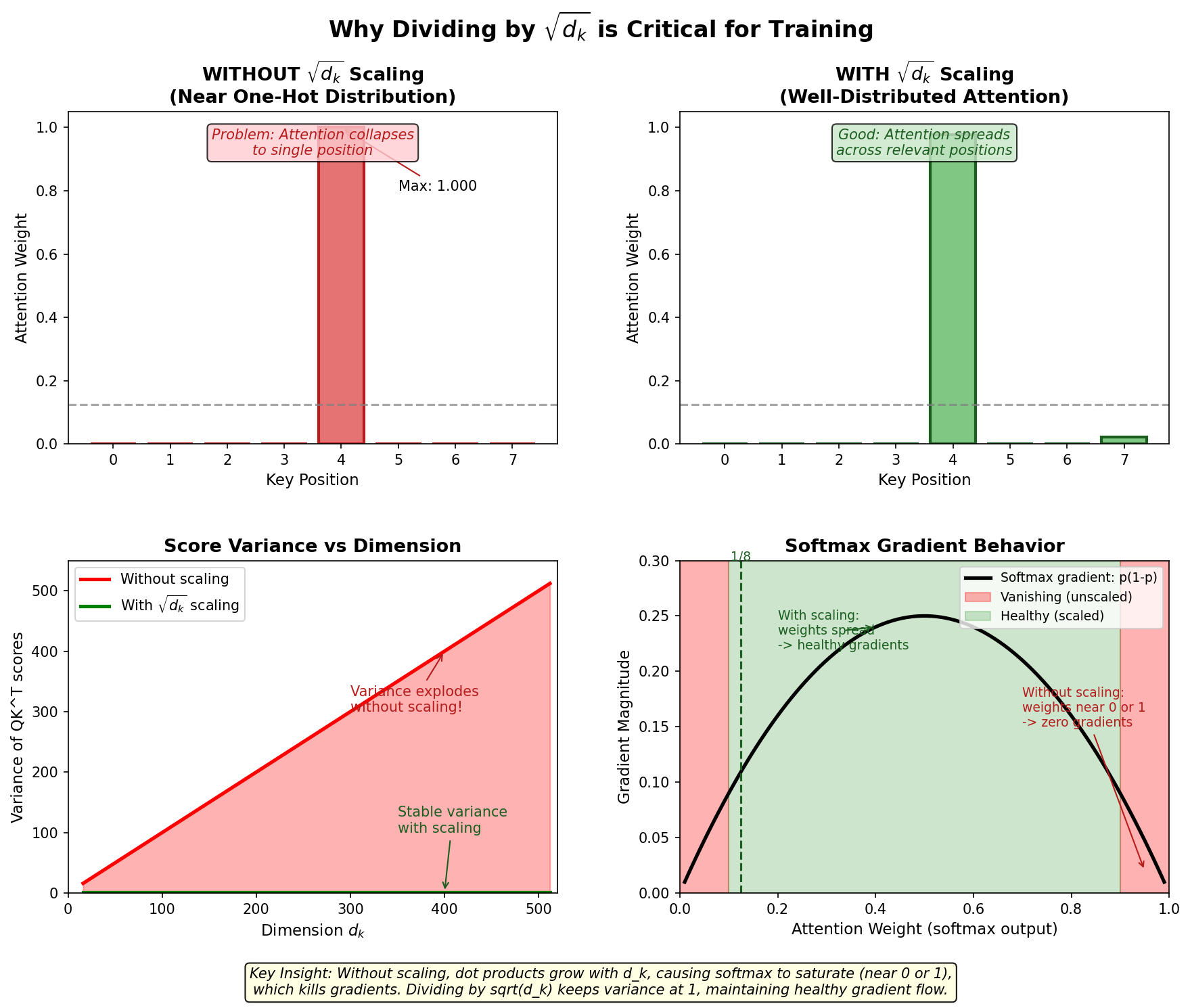
Q3: Why divide by √d_k in the attention formula? What goes wrong without it?

Expected Answer: The dot product QK^T produces values that scale with the dimension d_k. When d_k is large (e.g., 64), the dot products become very large numbers.

Without division:

• Large dot products push softmax into extreme regions (very peaked or flat)
• When peaked: gradients vanish (softmax(large_value) ≈ 1, gradient ≈ 0)
• When flat: sparse attention, no clear focus
• Optimization becomes difficult

With √d_k scaling:

• Dot products stay in reasonable range regardless of d_k
• Softmax maintains a well-behaved distribution with non-negligible gradients
• Stable training across different model sizes

Empirical observation: Without scaling, larger d_k models train much worse. This is why it's called "Scaled Dot-Product Attention."

Mathematical detail: The variance of a dot product between random vectors of dimension d_k is approximately d_k. Dividing by √d_k normalizes the variance to 1, keeping outputs in the regime where softmax gradients are largest.

Follow-up:

• "Would dividing by d_k work instead?" (Yes, but slightly worse empirically—√d_k is the theoretically motivated choice based on variance analysis)
• "Does this matter for small models?" (Matters more for large d_k; less critical for small models, but still best practice)

Common pitfall: Not understanding this is about gradient flow and optimization, not just "rescaling outputs."

---

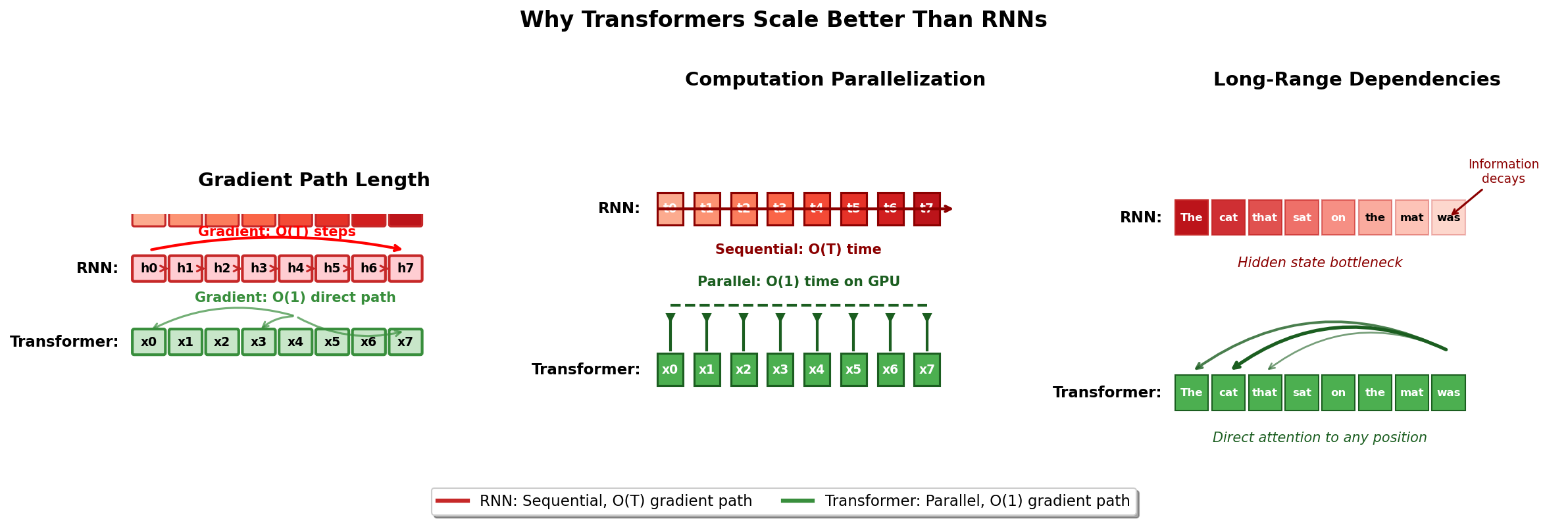
Q4: Why do transformers scale so much better than RNNs/CNNs? What's the architectural advantage?

Expected Answer: Three interconnected reasons:

1. Parallelization:

   • RNNs process sequentially (h_t depends on h_{t-1}), so you can't parallelize across time
   • Transformers compute all positions simultaneously, scaling to thousands of tokens per GPU
   • Training speedup: O(sequence_length) → O(1) for computation time (hardware permitting)

2. Gradient flow:

   • In RNNs, gradients multiply through many timesteps: ∂L/∂h_0 involves products of Jacobians
   • Vanishing gradients: ∏t (∂h_t/∂h_{t-1}) → 0 for long sequences
   • Transformers: Direct paths from each position to loss, distance-independent gradients
   • LSTMs help but don't fully solve this

3. Context window:

   • RNNs: Bottleneck of hidden state size limits context compression
   • Transformers: Every position can attend to every other position with full resolution
   • Enables learning long-range dependencies directly

Scaling laws consequence: Transformers follow power-law scaling: loss ∝ N^(-α), where N is parameters and α ≈ 0.07-0.08. This enabled the scaling trend from BERT (110M) → GPT-3 (175B) → GPT-4-class models (parameter count not publicly disclosed). RNNs don't scale this way.

Follow-up:

• "What about the O(n²) complexity of attention?" (True for inference, but training can use tricks like flash attention, sequence packing; still better than RNN's sequential bottleneck)
• "Don't CNNs also parallelize?" (Yes, but limited receptive field—need many layers to capture long-range dependencies, plus no explicit dependency modeling)

Common pitfall: Saying transformers are "just parallelizable"—the real power is combining parallelization with explicit global attention and superior gradient flow.

---

Q5: Describe multi-head attention. Why is it better than single-head?

Expected Answer: Multi-head attention runs multiple attention operations in parallel:

MultiHead(Q, K, V) = Concat(head_1, ..., head_h) W^O
where head_i = Attention(Q W_i^Q, K W_i^K, V W_i^V)

Each head has dimension d_v = d_model / num_heads. For d_model=512, h=8, each head is 64-dimensional.

Why multiple heads:

1. Representation diversity: Different heads can learn different types of relationships

   • Head 1 might focus on "subject-verb" dependencies
   • Head 2 might focus on "adjective-noun" dependencies
   • Head 3 might look at "pronoun-antecedent" relationships
   • No single head captures all pattern types optimally

2. Robustness: If one head gets stuck in local optima, others can still learn useful patterns

3. Computation is free: The total parameters and FLOPs don't increase (still d_model² parameters)—you're just reorganizing computation

4. Empirical validation: Ablations show removing heads hurts performance; analyzing attention reveals heads learn interpretable linguistic patterns

Example from BERT analysis:

• Some heads perform "redundant" attention (attend to same-sentence words)
• Others perform "positional" attention (attend to nearby tokens)
• Others are "rare" heads (specific to uncommon patterns)
• This diversity emerges without explicit supervision

Follow-up:

• "Could you have one huge attention head instead?" (Theoretically yes, but one attention matrix can't learn diverse patterns as easily)
• "How many heads should you use?" (Empirically 8-16 for most tasks; more recent models use fewer, larger heads)
• "Are all heads equally important?" (No—some heads are more specialized; some attend to specific patterns)

Common pitfall: Thinking heads are learned independently—they're trained jointly, so the diversity is emergent and discovered during training.

---

Q6: What's the computational complexity of the attention mechanism?

Expected Answer: Time complexity: O(n² d) where n is sequence length and d is embedding dimension

Breaking it down:

• Computing QK^T: Q is (n × d), K^T is (d × n) → matrix multiply is O(n² d)
• Softmax over n tokens: O(n²)
• Multiplying by V: O(n² d)
• Total: O(n² d)

Space complexity: O(n²) for storing attention weights

For comparison:

• RNN: O(n d²) time (d² for matrix multiplies at each step, n steps), O(d) space
• CNN with kernel k: O(n k d) time for k-sized convolution, O(d) space
• Transformers with n=2048, d=768: significantly more FLOPS than RNN with similar n, d

However:

• Transformers parallelize the n² operations across GPUs (wall-clock time is much better)
• Recent innovations reduce this:
  • Flash Attention: Same O(n² d) but 2-4x faster with optimized I/O
  • Sparse attention: Only attend to relevant tokens (local + strided), reducing to O(n k log n)
  • KV cache for inference: O(n d) for single token generation

Real-world impact:

• Training: GPU parallelization makes O(n²) tractable for n=2K-4K typical
• Inference: O(n² d) per token is expensive; KV caching makes it O(d) per token
• Length extrapolation: This is why long-context models (context window >100K) are recent innovations

Follow-up:

• "How does this affect training time and inference?" (Training is batch-parallelizable; inference is bottlenecked)
• "What are alternatives to reduce complexity?" (Sparse attention, local attention, linear attention approximations)
• "How does this compare to transformer alternatives?" (Mamba uses O(n d) with recurrence, but trains slower; Performer approximates attention)

Common pitfall: Confusing wall-clock time with theoretical FLOPS. Transformers have higher FLOP count but better hardware utilization.

---

Q7: Explain the layer normalization in transformers and why it's placed before/after attention.

Expected Answer: Layer normalization (LayerNorm) normalizes across the embedding dimension for each sequence position:

LayerNorm(x) = γ ⊙ (x - μ) / √(σ² + ε) + β

where μ and σ are computed across the d_model dimension (not batch dimension).

Two architectural choices:

1. Post-norm (original transformer): FF(LN(Attn(x) + x)) + FF output

   • Normalization applied to inputs of each module
   • Problematic for deep stacks (optimization becomes harder)

2. Pre-norm (modern standard): Attn(x) + LN(x), then FF(x) + LN(x)

   • Normalization applied to outputs before residual
   • Easier to train deep networks
   • Now used in most production models (BERT, GPT-2+, etc.)

Why LayerNorm instead of BatchNorm:

• BatchNorm normalizes across batch (doesn't work well with variable sequence lengths, small batches)
• LayerNorm normalizes within each example, independent of batch
• Makes sense for NLP where sequence lengths vary

Effect on training:

• Post-norm: Networks become "residual heavy"—stacking layers just adds more residuals, loses signal
• Pre-norm: Each layer processes normalized input, maintains signal flow through depth
• Pre-norm empirically trains deeper networks better (GPT-3 uses pre-norm exclusively)

Follow-up:

• "Why not use RMSNorm?" (RMSNorm is cheaper, empirically equivalent; used in modern models like Llama)
• "Could you remove LayerNorm?" (Yes, but training becomes unstable; empirically hurts performance)
• "Why not normalize at different granularities?" (Tried, but LayerNorm is the sweet spot)

Common pitfall: Thinking LayerNorm is "just batch normalization for NLP"—the difference is fundamental for deep networks.

---

Q8: Design a simple attention mechanism from scratch. What would you need to change?

Expected Answer: Start with the basic equation:

def scaled_dot_product_attention(Q, K, V, mask=None):
    d_k = Q.shape[-1]
    scores = matmul(Q, transpose(K)) / sqrt(d_k)  # Shape: (batch, seq_len, seq_len)

    if mask is not None:
        scores = scores + (mask * -1e9)  # Apply mask

    attention_weights = softmax(scores, dim=-1)  # Shape: (batch, seq_len, seq_len)
    output = matmul(attention_weights, V)  # Shape: (batch, seq_len, d_v)

    return output, attention_weights

Key implementation details:

1. Masking for causal/padding: Add large negative values to masked positions before softmax
2. Scaling: Always divide by √d_k, especially important for large d_k
3. Numerical stability: Subtract max from scores before softmax (log-sum-exp trick)
4. Gradient flow: Ensure softmax allows non-negligible gradients

Multi-head extension:

def multi_head_attention(Q, K, V, num_heads):
    # Project and split into heads
    Q = split_heads(linear(Q), num_heads)  # (batch, num_heads, seq_len, d_k)
    K = split_heads(linear(K), num_heads)
    V = split_heads(linear(V), num_heads)

    # Apply attention in parallel
    outputs = [scaled_dot_product_attention(Q_h, K_h, V_h) for Q_h, K_h, V_h in zip(Q, K, V)]

    # Concatenate heads and project
    concat = concatenate(outputs)  # (batch, seq_len, d_model)
    output = linear(concat)

    return output

Optimizations for production:

• Use fused kernels (Flash Attention) instead of vanilla softmax
• Reuse KV cache for inference
• Consider sparse attention for long sequences
• Profile bottlenecks (usually memory bandwidth, not compute)

Follow-up:

• "How would you handle variable length sequences?" (Padding + mask; or use bucket-based methods)
• "What about inference optimization?" (KV cache reduces computation from O(n²) per token to O(n) with cache)

Common pitfall: Forgetting the mask handling or incorrectly applying it before softmax normalization.

---

Architecture Questions

Q9: Walk me through a complete encoder block. What does each component do?

Expected Answer: An encoder block consists of:

Input (batch, seq_len, d_model)
    ↓
[Pre-norm] LayerNorm
    ↓
Multi-head Self-Attention → (batch, seq_len, d_model)
    ↓
+ Residual connection
    ↓
[Post residual] → x_attn
    ↓
[Pre-norm] LayerNorm
    ↓
Feed-Forward Network (two linear layers with ReLU/GELU)
    ↓
+ Residual connection
    ↓
Output (batch, seq_len, d_model)

Detailed breakdown:

1. LayerNorm before attention: Normalizes input to stable range, improves gradient flow
2. Self-attention: Each position attends to all positions (including itself), captures dependencies
3. Residual connection after attention: Helps gradients flow, enables deep stacking
4. LayerNorm before FFN: Again normalizes before feeding to nonlinear layer
5. FFN: Two linear layers with nonlinearity in between
   • First linear: d_model → d_ff (typically 4x larger)
   • ReLU/GELU: Introduces nonlinearity
   • Second linear: d_ff → d_model
   • Acts as dense feature transformation
6. Residual after FFN: Enables deep networks

Why both residuals are necessary:

• Attention residual: Prevents attention from collapsing to uniform distribution
• FFN residual: Prevents optimization issues in deep networks; acts as "feature highway"

Parameter count:

• Attention: 3d_model² (for Q, K, V projections) + 2d_model² (output projection) = 4d_model²
• FFN: 2d_model × d_ff + 2d_ff = 2d_ff(d_model + 1) ≈ 8d_model² (if d_ff = 4d_model)
• LayerNorm: 2d_model per norm (gamma, beta)
• Total: ~13d_model² parameters per encoder block

Follow-up:

• "Why is d_ff typically 4x d_model?" (Empirical finding; larger FFN improves capacity without hurting training)
• "Could you swap the order (FFN before attention)?" (No—attention should come first to mix information, then FFN to transform)
• "What if you remove the residuals?" (Training fails; gradients don't flow through deep networks)

Common pitfall: Not explaining why each component is necessary, or confusing pre-norm vs post-norm placement.

---

Q10: Explain pre-norm vs post-norm. Why do modern models use pre-norm?

Expected Answer:

Post-norm (original "Attention is All You Need"):

y = LayerNorm(x + SubLayer(x))

Normalization applied to the output (after residual)

Pre-norm (modern standard):

y = x + SubLayer(LayerNorm(x))

Normalization applied to the input (before sublayer)

Empirical differences:

Aspect	Pre-norm	Post-norm
Training stability	Better, easier to train deep models	Harder, needs careful LR scheduling
Depth limit	Can train 100+ layers	Typically limited to 24-48 layers
Warmup	Minimal warmup needed	Requires learning rate warmup
Initialization	Less sensitive	More sensitive to careful init
Gradient flow	Direct paths from output to input	Residuals accumulate

Why pre-norm is better:

1. Output residual effect: In post-norm, residuals dominate in deep networks

   • Let r_l = residual contribution, a_l = attention contribution
   • Deep network output: r_1 + r_2 + ... + r_L + (tiny attention signals)
   • The residuals overpower the learned features

2. Gradient magnitude: With pre-norm, gradients don't explode through residuals

   • ∂/∂x (x + f(LN(x))) has gradient 1 + ∂f/∂x
   • More stable than cascading residuals

3. Scaling behavior: Pre-norm doesn't require careful learning rate scaling as depth increases

   • Post-norm requires LR ∝ 1/sqrt(depth) for stability
   • Pre-norm is more forgiving

Empirical evidence:

• BERT (post-norm, 12 layers): Already showing training difficulty
• GPT-3 (pre-norm, 96 layers): Trains smoothly
• Modern LLMs (pre-norm): Standard choice

Follow-up:

• "What about layer-wise adaptive rate scaling (LARS)?" (Post-norm trick to help training, but pre-norm still better)
• "Is there a hybrid approach?" (Yes—deep norm, RMSNorm, etc., but pre-norm is the gold standard)

Common pitfall: Thinking the difference is "just where you put normalization"—the effect on optimization dynamics and depth scalability is profound.

---

Q11: Explain the decoder block and causal masking. Why is it different from encoder?

Expected Answer: A decoder block is similar to encoder, but with causal masking in self-attention:

Input (at position t, batch, d_model)
    ↓
[Pre-norm] LayerNorm
    ↓
Causal Self-Attention (attends only to positions ≤ t)
    ↓
+ Residual
    ↓
[Pre-norm] LayerNorm
    ↓
Feed-Forward Network
    ↓
+ Residual
    ↓
Output (batch, d_model)

Causal masking:

Attention scores for token at position t:
scores[t, :t+1] = valid (can attend to self and past)
scores[t, t+1:] = -∞ (masked, cannot attend to future)

After softmax: softmax(-∞) = 0, so future tokens get zero weight

Why causal masking:

• During training and inference, we generate one token at a time
• Token at position t should NOT see future tokens (t+1, t+2, ...) because they haven't been generated yet
• Without causal masking, the model would cheat: learning to copy from future tokens during training, then failing at inference

Encoder vs Decoder:

Aspect	Encoder	Decoder
Masking	No masking (sees full sequence)	Causal masking (only past + current)
Use case	Processing full input (bidirectional)	Generating one token at a time (unidirectional)
Training	Parallelizable (all positions together)	Parallelizable with masking
Inference	Process entire input at once	Autoregressive (one token per forward pass)
Example	BERT encoder block	GPT decoder block

Cross-attention (decoder-to-encoder): Decoders have an additional cross-attention layer:

... (self-attention on decoder)
    ↓
Cross-Attention:
  Q from decoder position t
  K, V from encoder output (full sequence, no masking)
  Allows decoder to attend to all encoder positions freely

Why it works:

• Decoder generates attending to past predictions (causal self-attention)
• Decoder also attends to full encoder output (cross-attention)
• Combination: Maintain auto-regressive generation while having access to full context

Follow-up:

• "Can you train decoder efficiently?" (Yes—parallelizable with causal mask; compute full matrix, mask before softmax)
• "What about bidirectional decoders?" (They break auto-regressive generation; used only in specific architectures like BERT masked LM)
• "How does inference differ?" (At inference, process one token at a time, reusing KV cache from previous tokens)

Common pitfall: Confusing causal masking with sequence masking (padding mask is different—it masks out padding tokens).

---

Q12: Explain cross-attention in sequence-to-sequence models. How does it differ from self-attention?

Expected Answer: Cross-attention allows the decoder to attend to encoder outputs:

Self-attention (encoder/decoder): Q, K, V all from same source
Cross-attention (decoder → encoder):
  Q from decoder
  K, V from encoder

Mechanism:

scores = (decoder_Q) @ (encoder_K)^T / √d_k
attention_weights = softmax(scores)
output = attention_weights @ encoder_V

Key differences:

Aspect	Self-attention	Cross-attention
Source	Q, K, V same	Q from decoder, K/V from encoder
Masking	Causal (decoder) or none (encoder)	No masking (full access)
Function	Relate positions within sequence	Relate decoder to encoder
Example	Position t attends to positions ≤t (causal)	Decoder position t attends to all encoder positions

Why cross-attention is critical:

1. Information flow: Encoder processes input, decoder needs to access it
2. Flexibility: Decoder can focus on different encoder positions for each output token
   • Generating word 5 might heavily attend to encoder words 2-3
   • Generating word 6 might attend to encoder words 7-8
3. Alignment mechanism: Cross-attention weights act as an alignment matrix (seen in machine translation, image captioning)

Example (Machine Translation):

Input: "The cat sat" (encoder processes, outputs context vectors)
Output generation (decoder with cross-attention):
  Token 1 "Le": attends heavily to "The" (determinant)
  Token 2 "chat": attends heavily to "cat" (noun)
  Token 3 "s'assit": attends to "sat" (verb)
Cross-attention weights form alignment between source and target!

Visualization:

Encoder outputs:     The  cat  sat  [context-aware]
                     ↑    ↑    ↑
Decoder position 1 "Le"—→ attends 95% to "The", 5% to cat
Decoder position 2 "chat" → attends 10% to "The", 80% to "cat", 10% to "sat"
Decoder position 3 "s'assit" → attends 5% to "The", 10% to "cat", 85% to "sat"

Follow-up:

• "What if encoder and decoder have different d_model?" (Use projection layers to match dimensions)
• "Is cross-attention necessary?" (Not strictly—you could concatenate encoder output to decoder input, but cross-attention is more efficient and interpretable)
• "How many cross-attention heads?" (Same as self-attention; allows diverse attention patterns)

Common pitfall: Confusing cross-attention with fusion or concatenation—cross-attention is specifically the mechanism for selective attention across sequences.

---

Training & Optimization Questions

Q13: Explain learning rate warmup. Why is it necessary in transformers?

Expected Answer: Learning rate warmup gradually increases the learning rate from 0 to a target value over initial steps:

if step < warmup_steps:
    lr = base_lr * (step / warmup_steps)
else:
    lr = base_lr (or decay)

Why transformers need warmup:

1. Gradient flow initialization: Early in training, gradients are uncontrolled

   • Random initialization means attention is uniform (all tokens equally weighted)
   • Gradients are large but noisy
   • Large learning rate early would cause divergence

2. Initialization-dependent dynamics: With post-norm (original transformer):

   • Gradients flow through residuals
   • Initial large residual contributions vs small attention contributions
   • Large LR amplifies instability
   • Warmup lets attention signals bootstrap

3. Adam optimizer effect: Even with adaptive learning rates, warmup helps

   • Early steps have high variance in gradient estimates
   • Warmup prevents overfitting to noisy initial gradients
   • Lets momentum and variance estimates stabilize

Empirical observation:

Without warmup: divergence, NaN loss
With warmup (10K steps): smooth training curve, optimal final loss

Parameters:

• Warmup fraction: typically 5-10% of total training steps
• For 1M steps: 50K-100K warmup steps
• Linear warmup: step/warmup_steps (simple, works well)
• Exponential warmup: less common

Interaction with scheduling:

Total learning rate = warmup_schedule(step) × base_schedule(step)

Step 0-warmup:      increasing from 0
Step warmup-end:    constant or cosine decay

Follow-up:

• "Do you always need warmup?" (Yes for large models, sometimes skippable for small models or with careful initialization)
• "What about different warmup types?" (Linear is standard; sometimes square-root warmup used)
• "Why not just start with small learning rate?" (Explicit warmup schedule is more predictable; small LR throughout is inefficient)

Common pitfall: Thinking warmup is "just for stability"—it's actually for initialization-dependent gradient dynamics.

---

Q14: Explain gradient flow and the challenges in training deep transformers.

Expected Answer: Deep networks face gradient challenges in backpropagation:

Vanishing gradients:

∂L/∂x_l = (∂L/∂x_L) × (∂x_L/∂x_{L-1}) × ... × (∂x_{l+1}/∂x_l)

Each Jacobian is typically < 1, so:
∂L/∂x_l ≈ product of L-l terms, each < 1
→ exponentially decays with depth

In transformers (pre-norm):

x_l = x_{l-1} + Attention(LN(x_{l-1}))
x_l = x_{l-1} + FFN(LN(x_{l-1}))

∂x_l/∂x_{l-1} = I + ∂Attention/∂x_{l-1}
∂x_l/∂x_{l-1} ≈ I + (small matrix) ≈ I (identity-like)

Gradient: ∂L/∂x_{l-1} = (∂L/∂x_l) × (I + small) ≈ ∂L/∂x_l

No decay! Gradients propagate backward evenly.

Why pre-norm helps:

• Residual connections have identity-like Jacobians
• Normalization before sublayer prevents gradient explosion
• Gradients remain O(1) throughout depth

Gradient explosion (opposite problem): Without normalization or clipping:

• Attention with large weights
• FFN with large weights
• Multiplication of Jacobians > 1 causes exponential growth

Modern solutions:

1. Layer normalization: Prevents scale explosion
2. Residual connections: Enables gradient flow with identity-like Jacobians
3. Pre-norm: Placed before sublayers to normalize inputs
4. Gradient clipping: Cap ||gradients|| to prevent explosions
5. Weight initialization: Careful scaling of initial weights

Empirical evidence:

• Deep RNNs (20+ layers): Nearly impossible to train
• Deep post-norm (48+ layers): Requires careful tuning
• Deep pre-norm (96 layers): Trains smoothly

Follow-up:

• "What about layer-wise LR scaling?" (Post-norm workaround, but pre-norm is better)
• "Does gradient clipping hurt?" (Necessary for stability, but high clip threshold preferred)
• "What about batch normalization?" (Doesn't work well for NLP due to variable sequence lengths)

Common pitfall: Saying "residuals solve the problem"—the full solution requires residuals + normalization + pre-norm placement.

---

Q15: What's the training objective for transformers? How does it differ across model types?

Expected Answer: The training objective depends on the model's task:

Causal language modeling (GPT):

Loss = -∑_t log P(x_t | x_1, ..., x_{t-1})

Predict next token given previous tokens. Standard cross-entropy on all positions.

Masked language modeling (BERT):

Randomly mask 15% of tokens:
  80% replace with [MASK]
  10% replace with random token
  10% keep original
Loss = -∑_{masked positions} log P(x_t | unmasked context)

Bidirectional context (encoder sees all except masked). Masked tokens are predicted conditionally independently given the unmasked context (no autoregressive dependency among the masked positions).

Sequence-to-sequence (T5):

Loss = -∑_t log P(y_t | y_1, ..., y_{t-1}, encoder_output)

Encoder processes input (no masking), decoder generates output (causal masking). Typical for translation, summarization.

Contrastive objectives (modern):

Loss = InfoNCE or similar
Maximize similarity to positive examples
Minimize similarity to negative examples
Used in models like CLIP, SIMCLR

Training details:

Model	Architecture	Masking	Loss	Use case
BERT	Encoder only	MLM (bidirectional)	Cross-entropy on masked	Pre-training, fine-tune for classification
GPT	Decoder only	Causal	Cross-entropy on all	Language generation, few-shot
T5	Encoder-decoder	Encoder: none, Decoder: causal	Cross-entropy on output	Conditional generation (translation, QA)
RoBERTa	Encoder	MLM improved	Cross-entropy	Better pre-training recipe

Pre-training vs fine-tuning:

• Pre-training: Large corpus, simple objective (MLM, causal LM)
• Fine-tuning: Task-specific data, task-specific loss
  • Classification: Cross-entropy on [CLS] token or pooled representation
  • QA: Span prediction (start/end positions)
  • NER: Token classification

Follow-up:

• "Why does BERT use MLM instead of causal LM?" (MLM provides bidirectional context, better for understanding tasks; causal LM for generation)
• "What's the auxiliary loss in T5?" (Denoising objective: corrupt input, reconstruct; similar to MLM but more general)
• "How do you handle variable-length sequences in the loss?" (Mask padding tokens, only compute loss on real tokens)

Common pitfall: Not distinguishing between pre-training and fine-tuning objectives; assuming all models use the same loss.

---

Model Variants & Scaling Questions

Q16: Compare BERT, GPT, and T5. What are the key differences and when would you use each?

Expected Answer:

Architecture comparison:

Aspect	BERT	GPT	T5
Architecture	Encoder-only	Decoder-only	Encoder-decoder
Masking	MLM (bidirectional)	Causal LM	Encoder: none, Decoder: causal
Pre-training	Masked language modeling	Causal language modeling	Denoising (text-to-text)
Depth/Params	12 layers, 110M	12-96 layers, 110M-175B	12 layers each, 220M-11B
Training time	Quick	Moderate-slow (depends on size)	Moderate (efficient ratio)

Detailed comparison:

BERT (Encoder-only):

• Strengths:
  • Bidirectional context (understands both directions)
  • Excellent for understanding tasks (classification, NER, QA)
  • Fast training, good efficiency
  • Strong baseline for smaller models
• Weaknesses:
  • Can't generate text naturally (trained on MLM, not causal)
  • Requires task-specific heads on top
  • Limited to classification-style tasks out-of-the-box
• Use when: Classification, NER, semantic similarity, smaller models

GPT (Decoder-only):

• Strengths:
  • Excellent at text generation (natural causal LM)
  • Few-shot learning (prompt-based)
  • Single unified architecture for all tasks
  • Scales extremely well (GPT-3 emergence of few-shot abilities)
• Weaknesses:
  • Requires prompt engineering for non-generation tasks
  • Slower inference (autoregressive generation)
  • MLM would be unidirectional
  • More parameters needed for same-quality understanding
• Use when: Text generation, few-shot learning, large-scale language models, user-facing applications

T5 (Encoder-decoder):

• Strengths:
  • Explicitly separates input encoding from output generation
  • Flexible: can handle any task as text-to-text
  • Good efficiency (separate encoder and decoder)
  • Works well for supervised tasks (translation, summarization, QA)
• Weaknesses:
  • More complex to implement and fine-tune
  • Requires paired input-output data
  • Slower than encoder-only for classification
• Use when: Machine translation, summarization, paraphrase generation, structured tasks with paired data

Practical decision tree:

Task type?
├─ Classification, tagging, understanding → BERT (or RoBERTa)
├─ Open-ended generation, chat → GPT (or similar decoder)
├─ Conditional generation (translation, summarization) → T5 (or encoder-decoder)
└─ Few-shot, in-context learning → GPT

Follow-up:

• "Can you use BERT for generation?" (Technically yes with modifications, but inefficient)
• "Can you fine-tune GPT for classification?" (Yes, but less efficient than BERT; encode, then classify)
• "Why not just use larger GPT for everything?" (GPT is more expensive; BERT is sufficient for many tasks)

Common pitfall: Thinking BERT and GPT are interchangeable; they're fundamentally different architectures for different purposes.

---

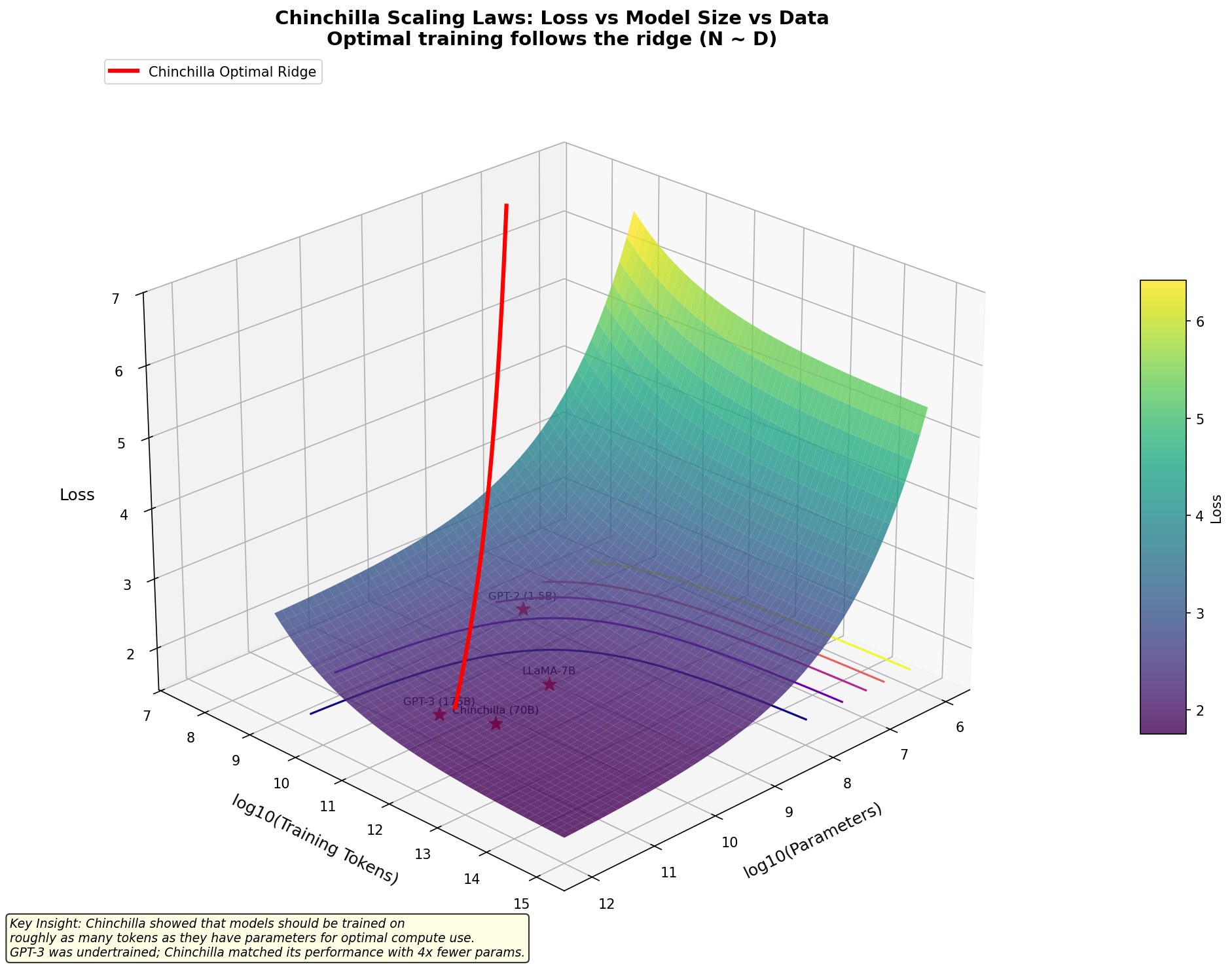
Q17: Explain scaling laws in transformers. Why do larger models work better?

Expected Answer: Empirical observations show predictable power-law relationships between model size, data size, and performance:

Chinchilla scaling laws (Hoffman et al., 2022):

Loss ≈ L(N, D) = E + A/N^α + B/D^β

where:
N = number of model parameters
D = number of training tokens
α ≈ 0.07, β ≈ 0.16 (approximately)
A, B, E = constants (depend on task)

Key insight: Optimal compute allocation

• Not N >> D or D >> N (token starving)
• Optimal: scale params and tokens at the same rate (each ∝ √C), with tokens ≈ 20× params
• E.g. for a fixed compute budget: 10M params × ~200M tokens (the token count should be roughly 20× the parameter count, not token-starved)

Why larger models work better:

1. Model capacity: Larger models have more parameters to fit data distribution

   • Small models quickly saturate (memorize training data)
   • Large models have room to generalize

2. Approximation theory: Universal function approximation

   • Transformers with more layers/heads can approximate more complex functions
   • Empirical: each doubling of parameters reduces loss by constant amount

3. Emergence of abilities:

   Tiny models (1M): Can memorize simple patterns
   Small models (100M): Learn basic linguistic structure
   Medium models (1B): Learn world knowledge, few-shot abilities
   Large models (100B+): In-context learning, reasoning, chain-of-thought

   These abilities don't appear linearly—they emerge at specific scales

4. Data efficiency: Larger models train on same data better than smaller models

   • Larger model can extract more information per token
   • But with scaling laws, beneficial to also scale data

Empirical evidence (GPT family):

GPT-1 (117M): Basic language model
GPT-2 (1.5B): Shows few-shot ability
GPT-3 (175B): Strong few-shot, reasoning, code
GPT-4 (estimated 1T+): Even stronger reasoning and planning

Each scale increase: new capabilities emerge

Practical implications:

• Scaling is predictable (can predict performance before training)
• Larger models are more sample-efficient (less overfitting)
• But larger models are more expensive to train and run
• Optimal training: scale model and data together

Follow-up:

• "What's the maximum useful model size?" (Unknown; no theoretical limit found yet; empirical trend continues)
• "How does compute scale differently for inference?" (Separate scaling laws; inference cost = d_model², requires optimization)
• "Do all architectures follow the same scaling laws?" (Different constants A, B, E; general shape similar)

Common pitfall: Thinking "bigger is always better"—actually, optimal scaling requires balancing model size, data size, and compute.

---

Q18: When would you use BERT vs GPT vs T5 in production? What are the practical trade-offs?

Expected Answer: Decision depends on task, latency, throughput, and cost requirements:

BERT in production:

Use for:

• Real-time classification (fraud detection, spam detection)
• Semantic search and similarity
• NER and tagging tasks
• Small models needed (mobile, edge devices)

Advantages:

• Fast inference (single forward pass, no generation)
• Small model size (110M-340M for BERT-base/-large)
• Low latency (10-50ms on CPU)
• Efficient serving (high throughput)

Trade-offs:

• Fixed output format (classification, tags)
• Requires task-specific fine-tuning
• Not suitable for open-ended generation

Example deployment:

User email → BERT classifier → spam/not spam (5ms)
Search query → BERT embeddings → similarity search (10ms)

GPT in production:

Use for:

• Text generation (chat, writing assistance)
• Few-shot learning (no fine-tuning needed)
• Complex reasoning tasks
• User-facing applications

Advantages:

• Unified model for all tasks
• Few-shot capability (prompt engineering)
• Strong performance on complex tasks
• Better reasoning abilities

Trade-offs:

• Slow inference (autoregressive generation, one token at a time)
• Large models (requires GPUs/TPUs)
• High latency (500ms-2s for typical generation)
• Expensive serving (high compute per request)

Example deployment:

User prompt → GPT → generate response (1-2 seconds)
High cost per request, suitable for premium features

T5 in production:

Use for:

• Conditional generation (translation, summarization)
• Structured tasks with clear input-output mapping
• Batch processing (lower-priority tasks)
• Cost-sensitive scenarios

Advantages:

• Efficient encoder-decoder (better than decoder-only for many tasks)
• Flexible (any task as text-to-text)
• Moderate inference cost
• Good quality-to-cost ratio

Trade-offs:

• More complex than BERT
• Slower than encoder-only for classification
• Slower than full-size GPT for generation
• Requires paired training data

Example deployment:

Documents → T5 summarizer → summaries (50ms per document)
Source text → T5 translator → target language (200ms per sentence)

Practical decision matrix:

Requirement	Best choice	Why
Real-time, <50ms latency	BERT	Encoder-only, no generation
Generation quality matters most	GPT-3/4	Superior reasoning
Cost-sensitive	BERT or small T5	Smaller models, efficient
Complex reasoning	GPT	Scaling laws show better reasoning
Translation/summarization	T5	Designed for conditional generation
Mobile deployment	Small BERT	~100M params fits on device
Batch processing	GPT or T5	Latency less critical

A/B comparison (realistic scenario - customer support):

Option 1: BERT classifier (intent detection)

• Model size: 100M
• Inference time: 20ms
• GPU cost: $50/day
• Throughput: 100 requests/sec

Option 2: GPT-style (generate response)

• Model size: 13B
• Inference time: 2s
• GPU cost: $500/day
• Throughput: 5 requests/sec

Decision: Use BERT for intent detection, then route to templates or GPT if needed

Follow-up:

• "How would you do A/B testing?" (Deploy both, measure latency/quality/cost tradeoff)
• "What about using smaller GPT models?" (GPT-2, Llama-2-7B can work; tradeoff quality vs speed)
• "Can you ensemble multiple models?" (Yes, but adds complexity; usually one model optimal)

Common pitfall: Choosing based on "latest" or "most powerful" rather than task-specific requirements.

---

Practical Application Questions

Q19: How do you fine-tune a pre-trained transformer for a specific task?

Expected Answer: Fine-tuning adapts a pre-trained model to a specific task with task-specific data:

High-level process:

1. Load pre-trained weights (encoder-only, decoder-only, or encoder-decoder)
2. Add task-specific head (classification layer, generation config, etc.)
3. Train on task-specific data with lower learning rate
4. Evaluate on validation set

For BERT (encoder-only):

# Load pre-trained BERT
model = BertForSequenceClassification.from_pretrained('bert-base-uncased', num_labels=2)

# Tokenize and prepare data
encoded = tokenizer(texts, padding=True, truncation=True)

# Fine-tune
optimizer = Adam(lr=2e-5)  # Much lower than pre-training!
for epoch in range(3):  # Usually 3-5 epochs
    for batch in train_data:
        outputs = model(input_ids, attention_mask, labels=batch_labels)
        loss = outputs.loss
        loss.backward()
        optimizer.step()

Key aspects:

• Learning rate: 2-5e-5 (much lower than pre-training)
• Epochs: 3-5 (not 100+; avoid overfitting)
• Batch size: 16-32 (depends on task data size)
• Warmup: Usually still helpful (5-10% of steps)

For GPT (decoder-only):

# Load pre-trained GPT-2
model = GPT2LMHeadModel.from_pretrained('gpt2')

# Fine-tune on task data (e.g., instructions)
# Just train language modeling objective on task examples
for batch in train_data:
    outputs = model(input_ids, labels=input_ids)  # Causal LM loss
    loss = outputs.loss
    loss.backward()
    optimizer.step()

Different from BERT:

• Reuse language modeling head (no new head)
• Reuse causal LM training objective
• May need prompt engineering

For T5 (encoder-decoder):

# Load pre-trained T5
model = T5ForConditionalGeneration.from_pretrained('t5-base')

# Fine-tune on paired input-output data
for source, target in train_data:
    input_ids = tokenizer(source, return_tensors='pt')['input_ids']
    label_ids = tokenizer(target, return_tensors='pt')['input_ids']
    outputs = model(input_ids, labels=label_ids)
    loss = outputs.loss
    loss.backward()
    optimizer.step()

Practical considerations:

1. Data size matters:

   • Few examples (< 1000): Risk overfitting, use smaller learning rate, early stopping
   • Medium examples (1K-100K): Standard fine-tuning works well
   • Many examples (> 100K): Can handle larger learning rate, more epochs

2. Domain shift:

   • Similar to pre-training domain: 3-5 epochs fine-tuning
   • Very different domain: More epochs needed, consider larger warmup

3. Early stopping: Monitor validation loss

   best_loss = float('inf')
   patience = 3
   for epoch in range(max_epochs):
       val_loss = validate()
       if val_loss < best_loss:
           best_loss = val_loss
           save_model()
           patience = 3
       else:
           patience -= 1
       if patience == 0:
           break  # Stop training

4. Hyperparameter tuning:

   • Learning rate: 2e-5 to 5e-5 typical
   • Batch size: 16, 32 (larger is often better but memory-limited)
   • Epochs: 3-5
   • Warmup: 10% of steps

Trade-offs (full fine-tuning vs parameter-efficient methods):

Method	Compute	Quality	Flexibility
Full fine-tuning	High	Best	Can adapt to any task
LoRA	Low	Near-best	Limited parameter updates
Prompt tuning	Very low	Worse	Limited to prompts
Few-shot	Very low	Baseline	No training

When to use each:

• Full fine-tuning: Sufficient compute, custom tasks
• LoRA: Limited GPU memory, many task-specific models
• Prompt tuning: Inference-only, few examples
• Few-shot: Rapid prototyping, no time for training

Follow-up:

• "How do you prevent catastrophic forgetting?" (Lower learning rate, early stopping, regularization)
• "Can you fine-tune on multiple tasks?" (Yes, multi-task fine-tuning—can help with similar tasks)
• "What about domain-specific pre-training?" (Pre-train on task domain, then fine-tune—works better)

Common pitfall: Using pre-training learning rate instead of lower fine-tuning rate, leading to instability or worse performance.

---

Q20: How would you deploy a transformer model in production? What are the key considerations?

Expected Answer: Production deployment requires careful planning across multiple dimensions:

Infrastructure decisions:

1. Hardware choice:
   • CPU-only: Suitable for small models (BERT), high latency acceptable (100-500ms)
   • GPU: Standard for inference, 10-100x speedup vs CPU
   • TPU/specialized: For very large models or high throughput
   • Quantization: Reduce model size, fit on smaller GPUs

Example trade-offs:

Model: BERT-base (110M params, 438MB)
Hardware: CPU single-threaded → 500ms latency
Hardware: GPU (NVIDIA A100) → 5ms latency
Hardware: Quantized CPU → 50ms latency (acceptable if cost-constrained)

2. Serving framework:

   • TensorFlow Serving: Production-ready, handles versioning
   • TorchServe: PyTorch-focused, good defaults
   • Hugging Face Inference Server: Optimized for transformers
   • Custom FastAPI: Lightweight, flexible
   • Triton Inference Server: Multi-model, complex scenarios

3. Scaling:

   • Single machine: 100-1000 requests/second
   • Load balancing: Multiple machines behind load balancer
   • Caching: Cache embeddings (BERT) or responses (GPT) if possible
   • Batching: Queue requests, batch inference for efficiency

Optimization techniques:

1. Model quantization:
   • FP32 → FP16 (half precision): 2x smaller, minimal quality loss
   • FP16 → INT8 (quantization): 4x smaller, slight quality loss
   • Distillation: Train small model to mimic large model

Example:

# Quantize BERT
model = torch.quantization.quantize_dynamic(
    model, {torch.nn.Linear}, dtype=torch.qint8
)
# Result: 110MB → 30MB, inference still 10x faster than quantized CPU

2. KV caching (generation):

   • Cache key-value tensors from previous generation steps
   • Avoid recomputing: O(n²) → O(n) per token
   • Memory trade-off: Faster inference

3. Prompt caching (if using LLMs):

   • Pre-compute and cache embeddings of system prompts
   • Reuse across requests

4. Batching and pipelining:

   • Batch multiple requests together
   • Pipeline multiple batches on GPU

Monitoring and reliability:

1. Performance monitoring:

   • Latency: p50, p95, p99 (not just mean)
   • Throughput: requests/second
   • GPU utilization: Should be 70-90%
   • Memory usage

2. Quality monitoring:

   • Predictions drifting from pre-training distribution
   • Accuracy on held-out test set (if applicable)
   • User feedback (if possible)

3. Error handling:

   • Graceful degradation (fallback to simpler model)
   • Timeouts (don't hang)
   • Circuit breakers (if service is down)

Example deployment architecture:

User requests
    ↓
Load balancer
    ↓
[API Server 1] [API Server 2] [API Server 3]
    ↓
[Model Server 1 - GPU] [Model Server 2 - GPU]
    ↓
[Model Cache] [Request Queue]

Cost optimization:

1. Model choice:

   • Smaller models (BERT-small): Lower cost
   • Appropriate model size for task
   • Trade-off: BERT-small 99% quality at 10% cost might be optimal

2. Inference optimization:

   • Quantization: 4x size reduction
   • Distillation: Use smaller model
   • Pruning: Remove unimportant weights

3. Infrastructure:

   • Spot instances: Cheaper but less reliable
   • Reserved instances: Cheaper for stable load
   • Auto-scaling: Match capacity to demand

Real-world example (semantic search service):

Requirement: 1M+ queries/day, <100ms latency, <$100/day

Solution:
1. Model: BERT-base (small but good quality)
2. Optimization: FP16 quantization (2x speedup)
3. Caching: Cache all query embeddings from past week (90% hit rate)
4. Hardware: Single GPU (NVIDIA T4 = $0.30/hour = $7/day)
5. Batching: Queue queries in 1-second windows (batch 100-200)
6. Result: 100-200 requests/second, <20ms latency

Cost breakdown:
- GPU: $7/day
- Bandwidth: $10/day
- Overhead: $5/day
Total: $22/day (under budget)

Follow-up:

• "How do you handle model updates?" (Blue-green deployment, canary rollout)
• "What about data privacy?" (On-premise vs cloud, encryption, PII handling)
• "How do you A/B test models?" (Shadow traffic, canary deployment)

Common pitfall: Deploying without considering inference optimization or cost, leading to runaway expenses or unacceptable latency.

---

Q21: Explain fine-tuning vs pre-training trade-offs. When should you do each?

Expected Answer:

Pre-training (from scratch):

• Objective: Learn language patterns from large corpus
• Data: Billions of tokens from diverse sources
• Time: Weeks-months on large compute clusters
• Cost: Millions of dollars (GPT-3 estimated ~$5M)
• Result: General-purpose model applicable to many tasks

Fine-tuning (on pre-trained):

• Objective: Adapt pre-trained model to specific task
• Data: Thousands to millions of tokens (task-specific)
• Time: Hours-days on modest compute
• Cost: Thousands to tens of thousands
• Result: Task-optimized model

When to pre-train from scratch:

1. Unique domain with no general transfer:

   • Example: Chemical compound modeling
   • General English BERT doesn't help much
   • Domain vocabulary and patterns are different
   • Justification: Massive domain-specific corpus available

2. Proprietary/sensitive data:

   • Can't use public models (data privacy)
   • Example: Financial institutions, healthcare
   • Must train on private data

3. Custom architecture:

   • Standard transformers don't fit your use case
   • Example: Custom sparse attention, different scaling
   • Can't use pre-trained weights

Realistic scenario - When pre-training is worthwhile:

Condition 1: Have > 10B tokens of high-quality domain data
Condition 2: Cannot use any public pre-trained model
Condition 3: Custom architecture needed
Condition 4: Have compute budget (millions of dollars)
Condition 5: Timeline allows (weeks-months)

Typical pre-training decision:
  If ANY condition is false, fine-tuning is better
  Most companies: Fine-tune (don't pre-train)

When to fine-tune:

1. Sufficient related pre-trained models exist:

   • Example: Customer support classification
   • Use BERT (general language understanding)
   • Fine-tune on support ticket corpus (10K examples)

2. Limited task-specific data (< 1M tokens):

   • Pre-training on 1M tokens: Poor quality, overfitting
   • Fine-tuning: Leverage pre-trained knowledge
   • Example: Medical diagnosis (limited labeled data)

3. Limited compute budget:

   • Fine-tuning: Days on single GPU
   • Pre-training: Weeks on 1000s of GPUs
   • Most practical choice for most companies

Trade-off analysis:

Factor	Pre-training	Fine-tuning
Data requirement	10B+ tokens	100K-1M tokens
Compute cost	Very high ($Ms)	Moderate ($Ks)
Time	Weeks-months	Hours-days
Final model quality	Best	Very good
Customization	Full	Limited to task
Starting point	Random	Pre-trained

Hybrid approach - Progressive training:

Step 1: Start with pre-trained (BERT, GPT, T5)
Step 2: Continue pre-training on domain corpus (intermediate)
Step 3: Fine-tune on task-specific data

Cost: Pre-train costs (~$100Ks) + fine-tune costs ($Ks)
Benefit: Better task performance than just fine-tuning
When: When you have significant domain-specific data (1B tokens)

Practical decision tree:

Have large domain-specific corpus (>10B tokens)?
├─ YES → Consider domain pre-training (if compute budget allows)
├─ NO → Use public pre-trained model
   ├─ Public model fits task?
   │ ├─ YES → Fine-tune
   │ └─ NO → Create custom pre-trained or modify architecture
   └─ Task-specific data available (>10K examples)?
     ├─ YES → Fine-tune on that data
     └─ NO → Few-shot or prompt engineering

Follow-up:

• "Is domain pre-training worth the cost?" (Usually no; unless domain shift is massive)
• "Can you warm-start pre-training?" (Yes, start with public model weights; usually saves 30-50% compute)
• "What about continual learning?" (Update model on new data; hard to avoid catastrophic forgetting)

Common pitfall: Under-appreciating the cost of pre-training and over-estimating the benefit vs fine-tuning.

---

Advanced / Follow-up Questions

Q22: Explain recent innovations in transformer optimization. What are RoPE and FlashAttention?

Expected Answer:

Rotary Position Embeddings (RoPE): Traditional positional encodings are additive. RoPE applies rotation matrices based on position.

Mechanism:

Traditional: x = x_embed + pos_embed
RoPE: Apply rotation matrix R(θ, pos) to query and key vectors

For complex representation:
R(θ, pos) rotates embedding in complex plane by angle pos×θ

Effect:
- Distance between positions has geometric meaning (rotation angle)
- Enables extrapolation: pattern of relative positions generalizes
- More efficient than additive PE (no extra parameters)

Why RoPE works better:

1. Relative position awareness: Relative distance has direct geometric meaning
2. Extrapolation: Pattern generalizes to longer sequences
3. Efficiency: No added parameters (unlike learned positional embeddings)
4. Compatibility: Works with KV caching (standard inference technique)

Adoption:

• LLaMA uses RoPE
• Used in most modern LLMs (GPT-4, Llama-2, Mistral)
• Displacing sinusoidal encodings in practice

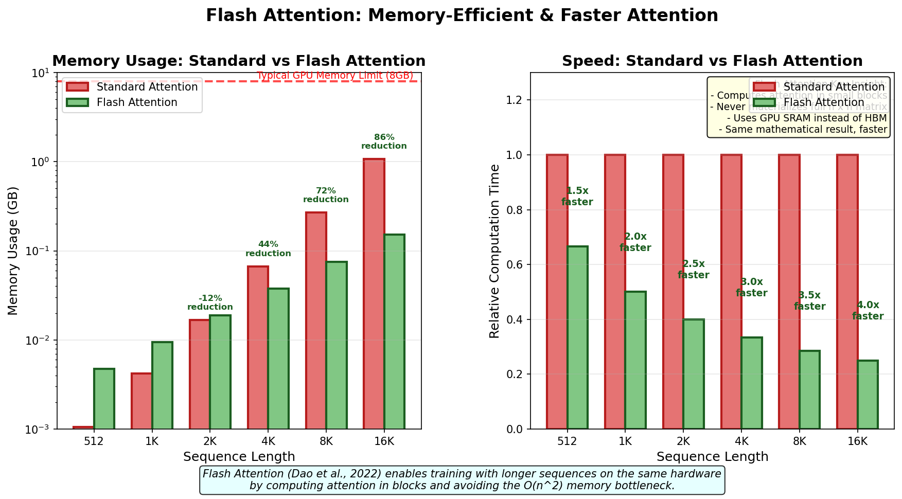
FlashAttention: Standard attention implementation:

1. Compute QK^T (n × n matrix on GPU memory)
2. Softmax (n × n matrix)
3. Multiply by V
Problem: For n=4096, n² = 16M values; doesn't fit in GPU cache
Solution: Move to GPU main memory; much slower

FlashAttention optimization:

Idea: Process attention in small blocks, recompute softmax statistics

Block 1: 128 tokens → 128×128 attention block fits in cache
Block 2: Next 128 tokens → Another cache-friendly block
...
Combine results (numerically stable)

Result: 2-4x faster on standard attention without losing accuracy

Why it matters:

• Same O(n² d) complexity, but much faster constant
• Enables longer sequences (4K → 8K-16K) at same GPU memory
• Backward pass also optimized (recompute instead of store)
• Now standard in most efficient implementations

Other recent innovations:

1. ALiBi (Attention with Linear Biases):

   • Instead of positional embeddings, add bias term to attention scores
   • Bias decreases with distance: attention(i,j) += -α × |i - j|
   • Advantage: Extrapolates to very long sequences (tested on 2M tokens)
   • Tradeoff: Slightly lower quality than RoPE for similar-length sequences

2. Sparse attention patterns:

   • Local attention: Only attend to nearby tokens (e.g., ±32 tokens)
   • Strided attention: Attend to every k-th token
   • Result: O(n k) instead of O(n²)
   • Used in models like Longformer

3. Multi-Query Attention:

   • Reduce KV cache size: all heads share same K, V
   • Multiple Q heads attend to shared K, V
   • Benefit: 4-8x faster inference with KV caching
   • Tradeoff: Slightly lower quality
   • Used in Llama-2

Practical implications:

Before Flash Attention (2023):
- Max sequence length: ~2048 (memory constraint)
- Inference cost: Linear in sequence length with KV cache
- Training: 4K sequences required large GPUs

After Flash Attention + optimizations:
- Max sequence length: 16K+ (same GPU)
- Inference: Multi-query attention reduces KV cache 4-8x
- Training: 4K-8K sequences on smaller GPUs

This enabled Claude, GPT-4, and modern long-context models

Follow-up:

• "How much does FlashAttention improve in practice?" (2-4x on standard transformers; varies by batch size and sequence length)
• "Does RoPE have any downsides?" (Extrapolation is better but not unlimited; still need to handle sequences much longer than training)
• "What about sparse attention trade-offs?" (Faster, but miss some long-range dependencies)

Common pitfall: Thinking "optimization = no quality loss"—some optimizations have quality/compute trade-offs.

---

Q23: How would you debug a transformer that's not learning?

Expected Answer: A model not learning is frustrating. Systematic debugging:

Step 1: Verify basic setup

# Can the model overfit on a single batch?
single_batch = get_batch(1)
for _ in range(10):
    loss = model(single_batch)
    loss.backward()
    optimizer.step()

# If loss doesn't decrease: bug in model or loss function
# If loss decreases: model is working, problem elsewhere

Step 2: Check data pipeline

# Are you loading the right data?
batch = next(iter(train_loader))
assert batch['input_ids'].shape == expected_shape
assert batch['labels'].min() >= 0  # Valid label indices

# Check for data leakage (test in train)
train_ids = set(train_dataset.ids)
val_ids = set(val_dataset.ids)
assert len(train_ids & val_ids) == 0  # Should be disjoint

Step 3: Verify loss computation

# Is loss decreasing during training?
# Plot loss curve—should be smooth downward slope

# Check loss magnitude
# Typical ranges:
#   Classification: loss = 0.69 (random BERT)
#   LM: loss = log(vocab_size) ≈ 10 (random GPT)
# If loss is way off, something's wrong

# Check gradient magnitudes
for name, param in model.named_parameters():
    if param.grad is not None:
        grad_norm = param.grad.norm()
        if grad_norm == 0:
            print(f"Zero gradient: {name}")  # Dead neuron

Step 4: Check learning rate

# Is learning rate too high or too low?
# Too high: loss diverges (NaN)
# Too low: loss flat or decreasing very slowly

# Try exponential search: 1e-6, 1e-5, 1e-4, 1e-3, 1e-2
# Plot loss vs learning rate; pick where loss decreases

# Also check warmup
# Without warmup: divergence in first steps (loss spikes to NaN)
# With warmup: loss decreases smoothly

Step 5: Verify model capacity

# Is model large enough?
# Doubling model size should improve loss
model_small = TransformerSmall()  # 100M params
model_large = TransformerLarge()  # 1B params

# Same data, same training
# If large model doesn't improve, data might be insufficient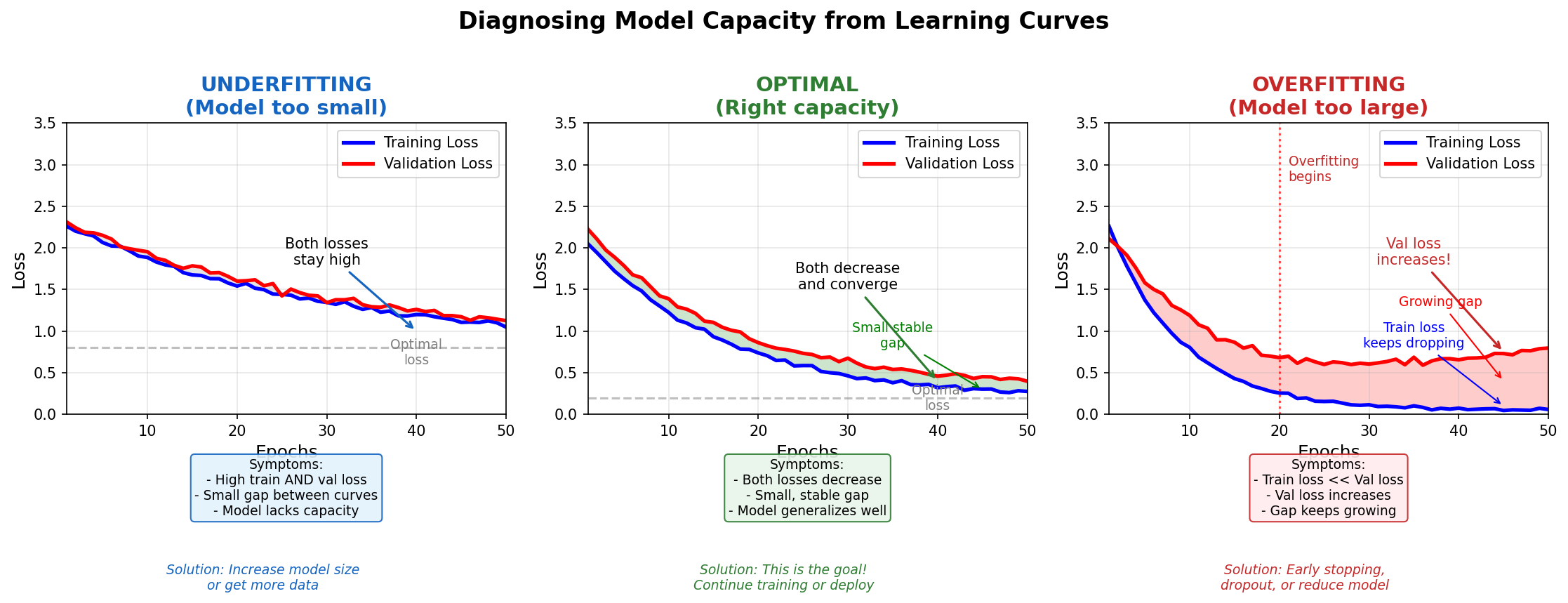

Step 6: Check for common bugs

Bug 1: Wrong tokenizer

# Tokenizer mismatch: training with one tokenizer, evaluating with another
# Check: token IDs should be consistent

Bug 2: Mask not applied correctly

# For padded sequences, are you masking out padding?
# Without mask: model trains on padding tokens (learns wrong patterns)
# Check: attention weights should be zero for padding tokens

Bug 3: Labels off-by-one

# Classification labels: should be 0 to num_classes-1
# Language modeling: should match token IDs (no special indexing)

Bug 4: No gradient flow to certain parameters

# Check: are all parameters receiving gradients?
# Use: retain_graph=True if needed, or check detach() calls

Step 7: Hyperparameter tuning

# Common issues:
# 1. Learning rate: too high (NaN) or too low (no improvement)
# 2. Batch size: too large (noise) or too small (unstable)
# 3. Warmup: too short (instability) or too long (slow convergence)
# 4. Weight decay: too high (underfitting) or too low (overfitting)

# Try standard values first:
#   LR: 2e-5 (fine-tuning), 1e-4 (training from scratch)
#   Batch size: 32-64 (depends on GPU)
#   Warmup: 10% of total steps
#   Weight decay: 0.01

Visualization techniques:

# Plot 1: Loss curve (should decrease)
# Plot 2: Gradient norms (should be stable, not exploding/vanishing)
# Plot 3: Learning rate schedule (should follow your schedule)
# Plot 4: Validation metrics (should improve with training)
# Plot 5: Attention weights (should not be uniform or all zeros)

Follow-up:

• "What if loss plateaus?" (Learning rate too low, model too small, data insufficient)
• "How do you know if overfitting?" (Validation loss increases while training loss decreases)
• "What about distributed training bugs?" (Synchronization issues, gradient accumulation mismatches)

Common pitfall: Changing multiple hyperparameters at once; isolate changes to identify the issue.

---

Q24: What are current limitations of transformers? What might replace them?

Expected Answer:

Current limitations:

1. Quadratic attention complexity:

   • O(n²) memory and compute for sequence length n
   • 4K context window is practical max; 100K+ is expensive
   • Inference is bottleneck for long sequences
   • Even with FlashAttention, fundamental O(n²) complexity remains

2. Lack of true reasoning:

   • Good at pattern matching and memorization
   • Struggle with novel reasoning tasks
   • Chain-of-thought helps but is ad-hoc, not fundamental
   • Can't reliably solve new problems unseen during training

3. Limited continual learning:

   • Catastrophic forgetting: training on new data hurts old performance
   • No mechanism to selectively retain/update knowledge
   • Requires careful fine-tuning to avoid degradation

4. Hallucinations and unreliability:

   • Generate confident but false information
   • No uncertainty quantification
   • No way to know confidence in predictions

5. Context window size:

   • Humans can reason about pages of text
   • Current LLMs lose track after 50-100K tokens
   • Recent models extend this, but still limited

What might replace transformers:

Recurrent alternatives (modern):

• Mamba: Linear time complexity O(n), selective state updates
• RWKV: Recurrence with transformers performance
• Advantage: O(n) inference, no quadratic bottleneck
• Trade-off: Slightly lower quality, harder to parallelize training
• Current status: Early promise, but transformers still dominant

State space models:

• S4, S5: Based on differential equations
• Advantage: O(n) complexity with theoretical grounding
• Current status: Research phase, not yet production-ready

Hybrid approaches:

• Don't replace entirely, but combine with transformers
• Use Mamba or RNN for long-term context
• Use transformer layers for complex reasoning
• Example: MoE (mixture of experts) transformers

Fundamental rethink:

• Current transformers: Fixed architecture, learned weights
• Future: Dynamic architecture, adaptive computation
• Example: Compute routing, conditional execution

Why transformers are hard to replace:

1. Empirical scaling: Proven to scale to trillions of parameters
2. Training efficiency: Parallelizable, GPU-friendly
3. Maturity: Well-understood, lots of tooling
4. Emergence: Shows emergent abilities with scale
5. Ecosystem: Huge number of pre-trained models

Realistic timeline:

2024-2025: Transformers dominant, incremental improvements (RoPE, FlashAttention)
2025-2027: Hybrid models explore (Mamba + Transformers)
2028+: New paradigm might emerge (but not guaranteed)

My bet: Transformers likely stay dominant for next 5+ years, with optimizations and hybrid approaches. A fundamental breakthrough might displace them, but it's not clear what that would be.

Follow-up:

• "Why would you switch from transformers?" (Context length, speed, or novelty in reasoning)
• "What about biological inspiration?" (Brains don't use self-attention; but unclear how to translate to large-scale learning)
• "Could you use transformers + Mamba?" (Yes—early experiments show promise for long-context tasks)

Common pitfall: Dismissing transformers as "solved"; they're actively researched with many open questions.

---

Quick Reference Card

Fundamental Formulas

Scaled Dot-Product Attention:

Attention(Q, K, V) = softmax(QK^T / √d_k) V

Multi-Head Attention:

MultiHead(Q, K, V) = Concat(head_1, ..., head_h) W^O
head_i = Attention(Q W_i^Q, K W_i^K, V W_i^V)

Feed-Forward Network:

FFN(x) = W_2 ReLU(W_1 x + b_1) + b_2
Usually: d_model → 4×d_model → d_model

Layer Normalization:

LayerNorm(x) = γ ⊙ (x - μ) / √(σ² + ε) + β

Sinusoidal Positional Encoding:

PE(pos, 2i) = sin(pos / 10000^(2i / d_model))
PE(pos, 2i+1) = cos(pos / 10000^(2i / d_model))

Learning Rate Warmup:

lr(step) = base_lr × min(1, step / warmup_steps)

Cross-entropy Loss (classification):

Loss = -∑_i log P(y_true_i)

Cross-entropy Loss (language modeling):

Loss = -∑_t log P(x_t | x_1, ..., x_{t-1})

Complexity Analysis

Operation	Time	Space
Self-attention (seq_len=n, d_k=d)	O(n² d)	O(n²)
FFN (d_model=d, d_ff=4d)	O(n d²)	O(d²)
Per transformer block	O(n² d)	O(n²)
Full encoder (L layers)	O(L n² d)	O(n²)
Inference per token (with KV cache)	O(n d)	O(n d)
Inference N tokens	O(N n d)	O(n d)

Model Comparison

Aspect	BERT	GPT	T5	Llama
Architecture	Encoder	Decoder	Enc-Dec	Decoder
Training	MLM	Causal LM	Denoising	Causal LM
Use case	Understanding	Generation	Conditional gen	All-purpose
Inference	Fast	Slow	Moderate	Slow
Size options	110M, 340M	125M-175B	60M-11B	7B-70B
Pre-training effort	Moderate	High	Moderate	Very high

Hyperparameter Ranges

Parameter	Typical Range	Notes
Learning rate (pre-training)	1e-4 - 1e-3	Depends on optimizer
Learning rate (fine-tuning)	1e-5 - 5e-5	Much lower than pre-training
Batch size	32-256	Larger is better, memory-limited
Warmup steps	5-10% of total	More for larger models
Epochs (fine-tuning)	3-5	Avoid overfitting
Max sequence length	512-4096	Longer is more expensive
d_model	512-2048	Scales with model size
num_heads	8-16	Usually d_model % num_heads = 0
d_ff	4 × d_model	Feed-forward hidden dimension
Dropout	0.1	Helps with regularization

Common Mistakes and How to Avoid

Mistake	Consequence	Fix
Using pre-training LR for fine-tuning	Instability, worse performance	Use 2e-5 to 5e-5 for fine-tuning
Not applying causal mask in decoder	Model cheats, fails at inference	Verify mask shape matches attention
Forgetting √d_k scaling	Gradient instability for large d_k	Always divide QK^T by √d_k
Using post-norm instead of pre-norm	Can't train deep networks	Use pre-norm in new models
Not handling padding correctly	Model learns padding patterns	Apply attention mask to padding
No learning rate warmup	Initial divergence	Warmup first 5-10% of steps
Too high learning rate	NaN losses, divergence	Start with smaller LR, increase if stable
Too low learning rate	Slow convergence, poor final loss	Learning rate doubling rule: test if loss improves
Mixing up tokenizers	Token ID mismatch, corrupted data	Use same tokenizer for train and eval
Not removing duplicates	Data leakage, overestimated performance	Check test set isn't in training data
Insufficient fine-tuning data	Poor performance	Need >100 examples; more is better
Too many epochs fine-tuning	Overfitting	Monitor validation loss, use early stopping

Interview Success Tips

1. Start broad, then narrow down

   • Begin with high-level explanation ("Attention computes weighted average...")
   • Then add details, wait for follow-up questions
   • Example: "Attention mechanism is..." → "Why scaling by √d_k?" → "What about multi-head?"

2. Always mention trade-offs

   • Accuracy vs latency
   • Model size vs performance
   • Cost vs quality
   • Demonstrating systems thinking impresses interviewers

3. Use examples

   • Abstract explanation: "Attention relates positions"
   • With example: "In 'The cat sat on the mat', position 2 (cat) attends to position 1 (The) more than position 6 (mat)"
   • Examples make explanations concrete and memorable

4. Test your knowledge

   • If you're not sure: "I believe... but let me think through this"
   • Showing your reasoning is better than guessing
   • Interviewers respect thoughtfulness

5. Connect concepts

   • Attention enables parallel computation
   • Parallel computation scales better than RNNs
   • Scaling laws show larger models are better
   • Showing connections demonstrates deep understanding

6. Know when to stop

   • Don't over-explain if interviewer seems satisfied
   • Watch for nods and "mm-hm" → good, keep going briefly
   • If they move to next question → stop and follow

7. Practice these answers

   • Read these Q&As multiple times
   • Practice explaining out loud (to yourself, to friend)
   • Practice writing code (implementations help crystallize understanding)
   • Practice connecting to examples (papers, models)

8. Recent developments matter

   • Mention RoPE, FlashAttention if relevant
   • Shows you follow the field
   • But don't over-emphasize—fundamentals matter more

9. Admission of uncertainty

   • "I'm not 100% sure, but..." is better than wrong confidence
   • Interviewers appreciate intellectual honesty
   • Shows maturity and understanding of limitations

10. Close with questions

    • "Does that answer your question?" → gives interviewer chance to probe
    • Shows you're engaged
    • Allows for deeper follow-ups

Final Reminders

• Transformers are powerful but not magic: They're carefully designed combinations of known techniques (attention, residuals, normalization)
• Scaling laws are real: Bigger models do better, predictably
• Practical considerations matter: Cost, latency, deployment often matter more than 1% accuracy improvement
• Recent innovations are incremental: RoPE, FlashAttention improve efficiency, not fundamentals
• The field is still young: Open questions remain (true reasoning, continual learning, efficiency)
• Your role in an interview: Show you understand why transformers work, not just that they do

---

End of Module 10: Interview Questions Compendium

This module synthesizes all previous modules (1-9) into interview-ready Q&A format. Review this material multiple times, practice explaining answers aloud, and most importantly, understand the why behind each answer. Interviewers value understanding over memorization.