Perceptrons & MLPs

The building blocks of neural networks — from single neurons to universal function approximators

---

The Perceptron

The perceptron, introduced by Frank Rosenblatt in 1958, is the simplest neural network unit. It models a biological neuron that "fires" when its inputs exceed a threshold.

Mathematical Formulation

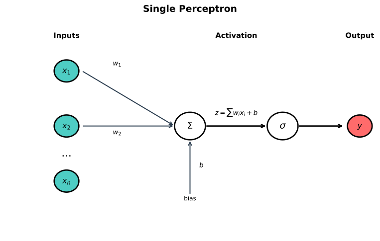
A perceptron computes a weighted sum of inputs and applies a step function:

$$y=\text{sign}(\mathbf{w}\cdot \mathbf{x}+b)=\text{sign}(\sum _{i=1}^n{w}_i{x}_i+b)$$

Where:

• $\mathbf{x}=[x_1,x_2,\dots ,x_n]$ are input features
• $\mathbf{w}=[w_1,w_2,\dots ,w_n]$ are learnable weights
• $b$ is the bias term
• $\text{sign}(z)$ returns +1 if $z>0$, else -1

The Perceptron Learning Algorithm

The perceptron learns through a simple update rule:

For each training example (x, y):
    prediction = sign(w · x + b)
    if prediction != y:
        w = w + y * x
        b = b + y

Key insight: The perceptron converges to a solution in finite steps if the data is linearly separable. This is the Perceptron Convergence Theorem.

What a Perceptron Can Learn

A single perceptron can only learn linear decision boundaries — hyperplanes that separate classes:

• AND gate: learnable
• OR gate: learnable
• NOT gate: learnable

---

The XOR Problem

In 1969, Minsky and Papert showed that a single perceptron cannot learn XOR, dealing a major blow to neural network research.

Why XOR Fails

$x_1$	$x_2$	XOR
0	0	0
0	1	1
1	0	1
1	1	0

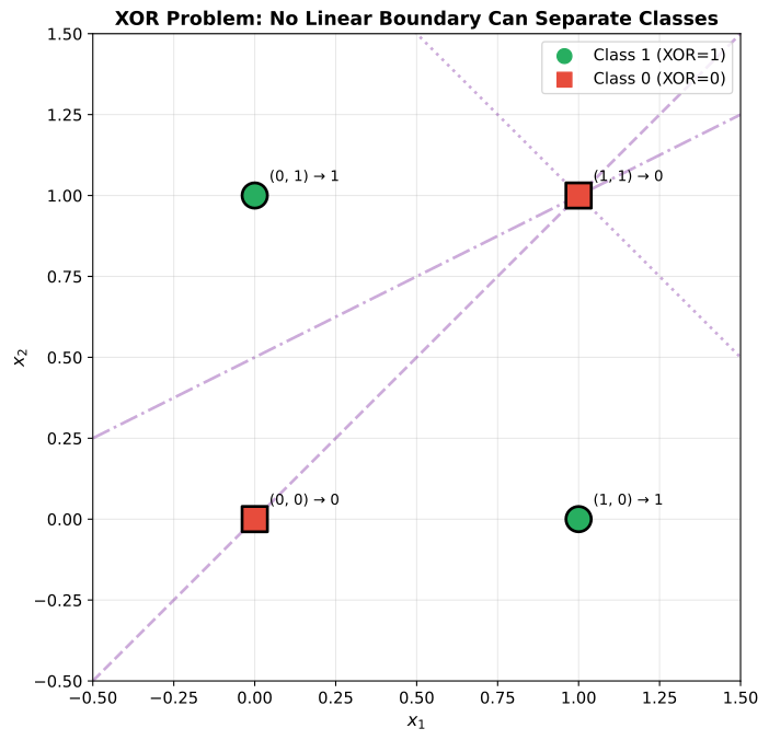
No single line can separate the positive (1) examples from the negative (0) examples. XOR is not linearly separable.

The Solution: Hidden Layers

By adding a hidden layer, we can first transform the input space to make it linearly separable, then separate with a second layer.

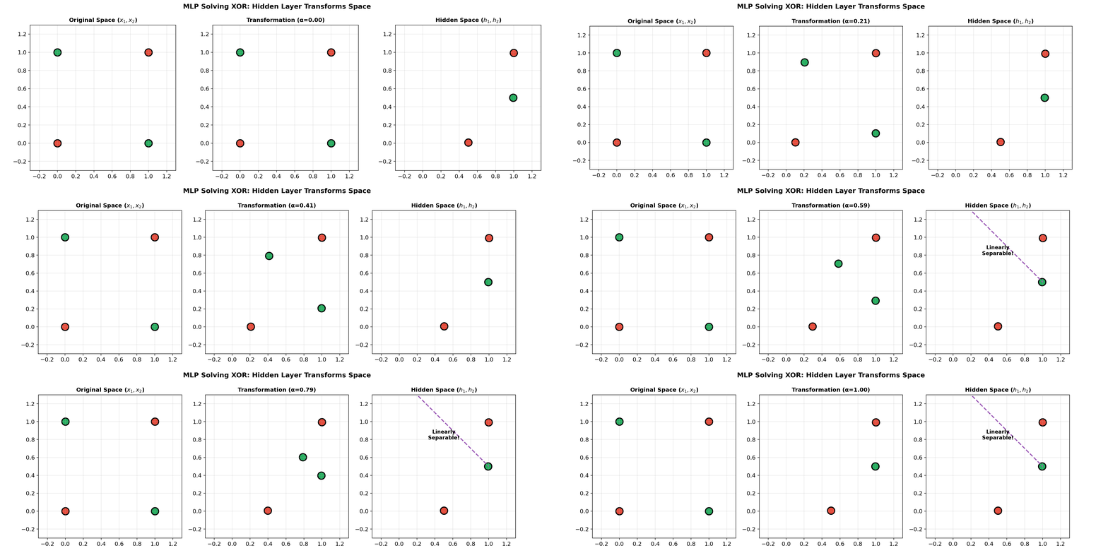
The hidden layer learns to map:

• $(0,0)\to$ point A
• $(0,1)\to$ point B
• $(1,0)\to$ point C
• $(1,1)\to$ point D

In this transformed space, the classes become linearly separable.

---

Multi-Layer Perceptrons (MLPs)

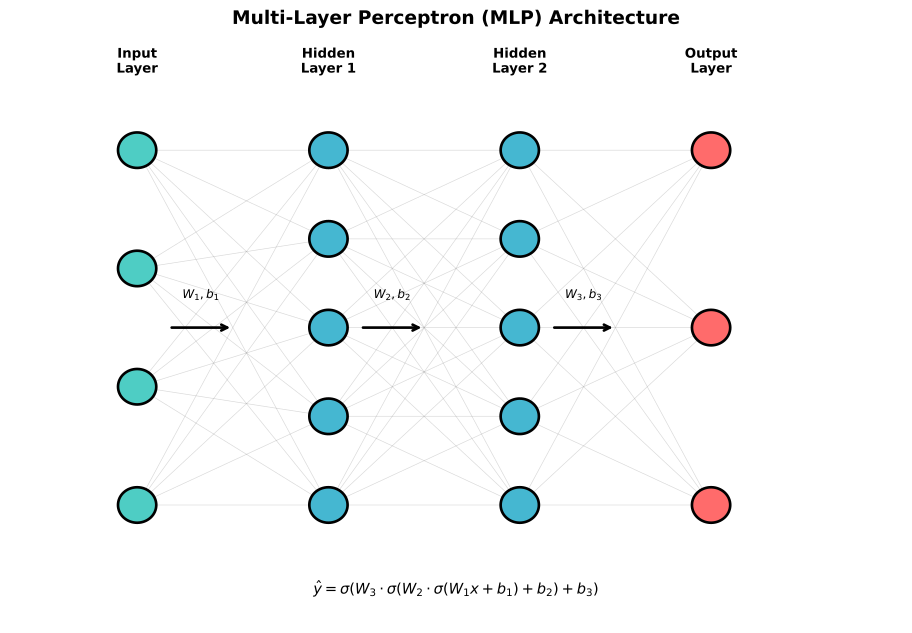
An MLP stacks multiple layers of neurons, each fully connected to the next.

Architecture

Input Layer    Hidden Layer(s)    Output Layer
    x₁  ─────┐
    x₂  ─────┼──►  h₁  ───┐
    x₃  ─────┤     h₂  ───┼──►  y₁
    ...      │     h₃  ───┤     y₂
    xₙ  ─────┘     ...    │     ...
                   hₘ  ───┘     yₖ

Mathematical Formulation

For an L-layer MLP:

$${\mathbf{z}}^{[l]}={\mathbf{W}}^{[l]}{\mathbf{a}}^{[l-1]}+{\mathbf{b}}^{[l]}$$$${\mathbf{a}}^{[l]}=g({\mathbf{z}}^{[l]})$$

Where:

• ${\mathbf{a}}^{[0]}=\mathbf{x}$ (input)
• $g(\cdot )$ is the activation function
• ${\mathbf{a}}^{[L]}=\hat{\mathbf{y}}$ (output)

Why Depth Matters

Property	Wide (1 hidden layer)	Deep (many layers)
Expressiveness	Universal approximator	Also universal approximator
Efficiency	May need exponentially many neurons	Often fewer parameters for same function
Representation	Flat features	Hierarchical features
Training	Easier optimization	Harder (vanishing gradients)

Key insight: Deep networks learn hierarchical representations — early layers learn simple features (edges), later layers learn complex features (objects).

---

Universal Approximation Theorem

Theorem: A feedforward network with a single hidden layer containing a finite number of neurons can approximate any continuous function on compact subsets of ${\mathbb{R}}^n$, to any desired precision.

What This Means

• MLPs are universal function approximators
• A single hidden layer is theoretically sufficient
• The theorem says nothing about:
  • How many neurons are needed
  • How to find the right weights
  • Whether training will converge

Practical Implications

In practice, deep networks (multiple layers) are often more efficient than wide networks (single huge layer) for learning complex functions.

---

Decision Boundaries

Hidden layers allow networks to learn complex, non-linear decision boundaries.

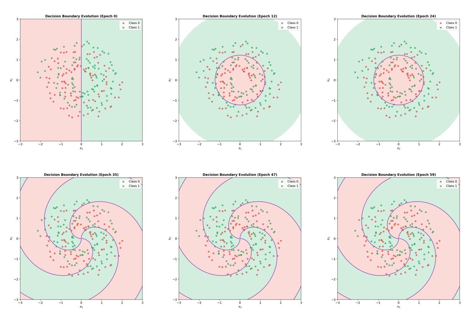
Network Depth	Decision Boundary
0 hidden layers	Linear (hyperplane)
1 hidden layer	Piecewise linear / smooth curves
2+ hidden layers	Arbitrarily complex shapes

How Hidden Layers Create Complex Boundaries

Each hidden neuron creates a linear boundary. The combination of many linear boundaries, composed through layers, creates complex non-linear boundaries.

---

Forward Pass Implementation

import numpy as np

def forward_pass(X, weights, biases, activation='relu'):
    """
    Forward pass through an MLP.

    Args:
        X: Input data (batch_size, input_dim)
        weights: List of weight matrices
        biases: List of bias vectors
        activation: Activation function ('relu', 'sigmoid', 'tanh')

    Returns:
        Output and cached activations for backprop
    """
    activations = {'relu': lambda z: np.maximum(0, z),
                   'sigmoid': lambda z: 1 / (1 + np.exp(-z)),
                   'tanh': np.tanh}

    g = activations[activation]

    a = X
    cache = [a]

    for W, b in zip(weights[:-1], biases[:-1]):
        z = a @ W + b
        a = g(z)
        cache.append(a)

    # Output layer (linear for regression, softmax for classification)
    z = a @ weights[-1] + biases[-1]
    output = z  # or softmax(z) for classification

    return output, cache

---

Interview Questions

Q1: "Why can't a single perceptron solve XOR?"

A single perceptron can only learn linear decision boundaries (hyperplanes). XOR is not linearly separable — no single line can separate the positive examples ((0,1), (1,0)) from the negative examples ((0,0), (1,1)).

The solution is adding a hidden layer. The first layer transforms the input space to make the classes linearly separable. For example, one hidden neuron can compute $h_1=(x_1\text{ AND }{x}_2)$ and another $h_2=(x_1\text{ OR }{x}_2)$. In this transformed space $(h_1,h_2)$, XOR becomes $h_2\text{ AND NOT }{h}_1$, which is linearly separable.

This illustrates the key insight: hidden layers learn representations that make the problem easier for subsequent layers.

Q2: "What is the universal approximation theorem and what are its limitations?"

The theorem states: A feedforward network with a single hidden layer can approximate any continuous function on a compact domain to arbitrary precision, given enough hidden neurons and appropriate activation functions.

Limitations:

1. Doesn't specify how many neurons — may need exponentially many
2. Doesn't say how to find weights — just that they exist
3. Doesn't guarantee training will converge — optimization may fail
4. Doesn't address generalization — only approximation on training domain

Practical implication: Deep networks often achieve the same approximation with fewer parameters than wide networks, and they learn more meaningful hierarchical features.

Q3: "How does adding depth help neural networks?"

Depth enables hierarchical feature learning:

• Layer 1: Low-level features (edges, textures)
• Layer 2: Mid-level features (shapes, parts)
• Layer 3+: High-level features (objects, concepts)

Efficiency: Some functions require exponentially many neurons in a shallow network but only polynomial neurons in a deep network.

Trade-off: Deeper networks are harder to train due to vanishing gradients, but techniques like residual connections, normalization, and careful initialization have largely solved this.

Example: A 10-layer CNN can recognize ImageNet objects with ~25M parameters. A 1-layer network would need vastly more.

---

Key Takeaways

1. Perceptrons are linear classifiers — they can only learn linearly separable problems.

2. The XOR problem demonstrates the need for hidden layers to learn non-linear decision boundaries.

3. MLPs are universal approximators — but the theorem doesn't guarantee efficient learning.

4. Depth enables hierarchical representations — each layer builds on features from the previous layer.

5. Hidden layers transform the input space — making complex problems linearly separable at the output layer.