Advanced RL Topics

Beyond single-agent online learning — multi-agent, offline, and model-based RL

---

Overview

Standard RL assumes a single agent learning through online interaction with an environment. Real-world applications often require extensions: multiple agents learning together, learning from fixed datasets without exploration, or building predictive models of the environment. This module covers these advanced paradigms that frequently appear in ML interviews.

---

Multi-Agent Reinforcement Learning (MARL)

The Multi-Agent Setting

In MARL, multiple agents interact within a shared environment. Each agent $i$ observes state $s_t$, takes action $a_t^i$, and receives reward $r_t^i$. The key challenge: non-stationarity. From agent $i$'s perspective, other agents are part of the environment, but they are also learning and changing their policies.

The joint action space grows exponentially: with $n$ agents and $|A|$ actions each, the joint space has $|A{|}^n$ actions.

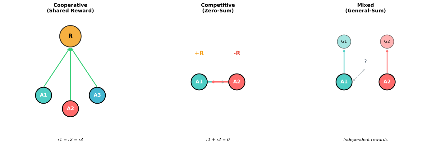
Cooperative vs Competitive

Setting	Reward Structure	Examples	Challenge
Cooperative	Shared reward: $r^1=r^2=...=r^n$	Robot teams, multi-robot navigation	Credit assignment
Competitive	Zero-sum: $r^1+r^2=0$	Games (Go, Chess, Poker)	Exploitability
Mixed	General-sum: independent rewards	Traffic, markets	Equilibrium selection

Centralized Training, Decentralized Execution (CTDE)

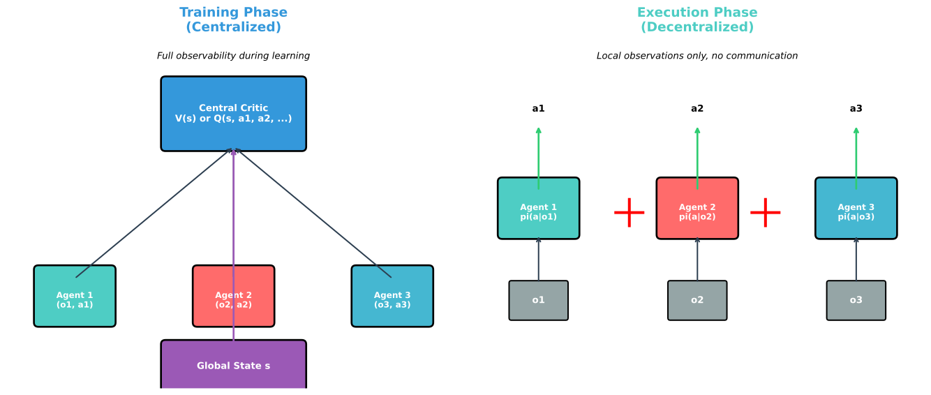
The dominant paradigm in MARL addresses non-stationarity during training while maintaining practicality during deployment:

Training Phase (Centralized):

• Access to all agents' observations and actions
• Can use global state information
• Enables stable learning with full information

Execution Phase (Decentralized):

• Each agent acts only on its local observation
• No communication required between agents
• Practical for real-world deployment

Key MARL Algorithms

Independent Q-Learning (IQL): Each agent learns independently, treating others as environment. Simple but ignores coordination.

QMIX: Learns a mixing network that combines individual Q-values into a joint Q-value, ensuring Individual-Global-Max (IGM) property:

$$Q_{tot}(s,\mathbf{a})=f_{mix}(Q_1(s,a_1),...,Q_n(s,a_n))$$

The mixing network must be monotonic in individual Q-values to ensure consistent argmax.

MAPPO: Multi-Agent PPO with a centralized critic. The critic $V(s)$ uses global state, while actors ${\pi }_i(a_i|o_i)$ use local observations.

---

Offline Reinforcement Learning

The Offline Setting

Online RL: Agent collects data by interacting with environment, learns from that data, collects more data, iterates.

Offline RL: Agent has a fixed dataset $\mathcal{D}=\{(s,a,r,s^{\prime })\}$ collected by some behavior policy ${\pi }_{\beta }$. No additional interaction allowed.

This setting is critical for:

• Healthcare (can't experiment on patients)
• Autonomous driving (can't cause accidents)
• Industrial systems (can't disrupt operations)

The Distribution Shift Problem

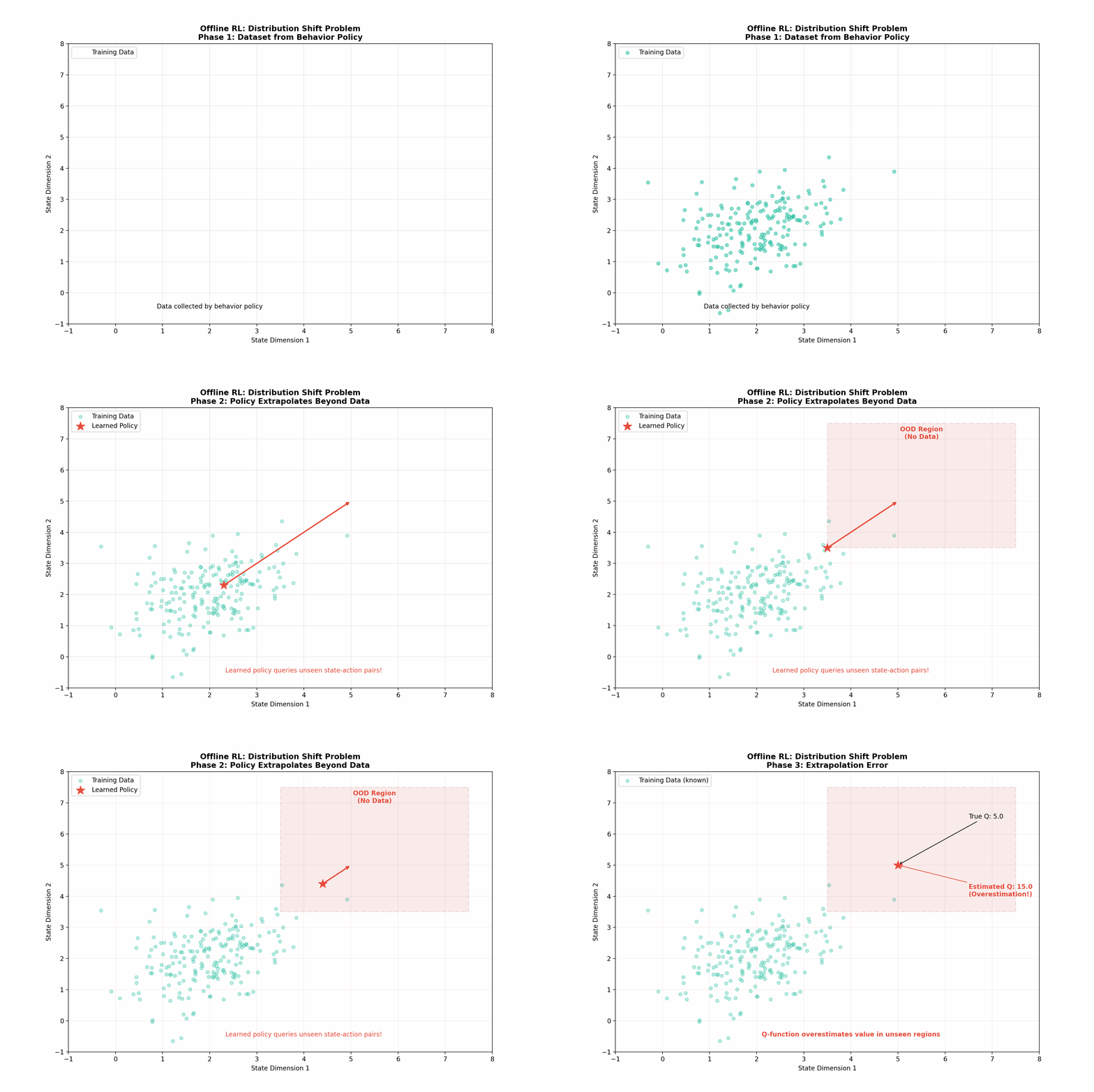
The fundamental challenge in offline RL is distribution shift. The learned policy $\pi$ may query the Q-function at state-action pairs $(s,a)$ not present in the dataset $\mathcal{D}$.

$$\text{OOD Error}={\mathbb{E}}_{(s,a)\sim \pi }[Q(s,a)]-{\mathbb{E}}_{(s,a)\sim \mathcal{D}}[Q(s,a)]$$

Standard Q-learning assumes the agent can correct errors through exploration. Without exploration, extrapolation errors compound:

1. Q-function overestimates value for unseen action $a^{\prime }$
2. Policy selects $a^{\prime }$ because of overestimation
3. No data to correct the error
4. Error amplifies in subsequent bootstrapping

Conservative Q-Learning (CQL)

CQL addresses distribution shift by adding a conservative regularizer to push down Q-values for out-of-distribution actions:

$${\mathcal{L}}_{CQL}={\mathbb{E}}_{s\sim \mathcal{D}}[\log \sum _a\exp (Q(s,a))]-{\mathbb{E}}_{(s,a)\sim \mathcal{D}}[Q(s,a)]+{\mathcal{L}}_{TD}$$

The first term (logsumexp) is minimized by reducing Q-values for all actions, while the second term prevents Q-values from collapsing for in-distribution actions.

Intuition: Learn a lower bound on the true Q-function. This ensures the policy doesn't overestimate the value of unseen actions.

Implicit Q-Learning (IQL)

IQL avoids querying Q-values for actions not in the dataset by using expectile regression:

$${\mathcal{L}}_{IQL}={\mathbb{E}}_{(s,a,s^{\prime })\sim \mathcal{D}}[L_{\tau }(r+\gamma V(s^{\prime })-Q(s,a))]$$

where $L_{\tau }$ is the asymmetric expectile loss:

$$L_{\tau }(u)=|\tau -\mathbf{1}(u<0)|\cdot u^2$$

With $\tau >0.5$, this implicitly performs policy improvement without explicit maximization over actions.

---

Model-Based Reinforcement Learning

Model-Free vs Model-Based

Aspect	Model-Free	Model-Based
Learns	Policy $\pi$ or Q-function directly	Dynamics model $\hat{T}(s'
Sample Efficiency	Low (needs many interactions)	High (can plan with model)
Computation	Low per step	High (planning required)
Asymptotic Performance	Can be optimal	Limited by model accuracy

World Models

A world model learns to predict environment dynamics and rewards:

$${\hat{s}}_{t+1}=f_{\theta }(s_t,a_t),{\hat{r}}_t=g_{\theta }(s_t,a_t)$$

Modern world models often operate in a learned latent space:

1. Encoder $e_{\varphi }$: Map observation to latent state $z_t=e_{\varphi }(o_t)$
2. Dynamics $f_{\theta }$: Predict next latent state ${\hat{z}}_{t+1}=f_{\theta }(z_t,a_t)$
3. Reward $g_{\psi }$: Predict reward ${\hat{r}}_t=g_{\psi }(z_t,a_t)$
4. Decoder $d_{\xi }$: Reconstruct observation (optional) ${\hat{o}}_t=d_{\xi }(z_t)$

Planning with Learned Models

Once a model is learned, several planning strategies exist:

Model Predictive Control (MPC):

1. At state $s_t$, sample action sequences $\{a_t,...,a_{t+H}\}$
2. Roll out each sequence using the learned model
3. Execute first action of best sequence
4. Replan at next timestep

Dyna-style Learning:

• Use real data to update both model and policy
• Generate synthetic rollouts from model
• Update policy on synthetic data

Dreamer:

• Learn world model in latent space
• Learn policy entirely within "dreams" (model rollouts)
• Only use real environment for model learning

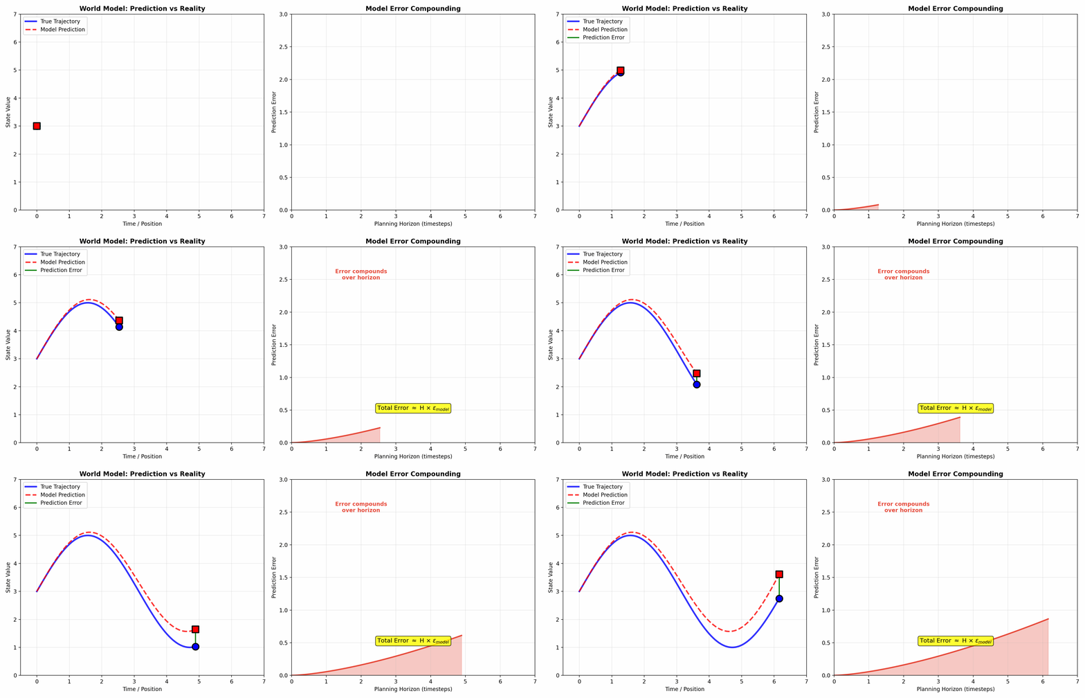
Model Error Compounding

The critical challenge in model-based RL: error compounding. Small model errors at each step accumulate over long horizons:

$$\text{Total Error}\approx H\cdot {ϵ}_{model}$$

where $H$ is the planning horizon and ${ϵ}_{model}$ is per-step model error.

Mitigation strategies:

• Short planning horizons (MPC)
• Ensemble models (uncertainty quantification)
• Dyna-style mixing of real and simulated data

---

Hierarchical Reinforcement Learning

The Temporal Abstraction Problem

Complex tasks require reasoning at multiple timescales. Navigating a city involves high-level decisions (which route?) and low-level control (steering, braking).

Options Framework

An option $\omega =(I_{\omega },{\pi }_{\omega },{\beta }_{\omega })$ consists of:

• Initiation set $I_{\omega }$: States where option can start
• Policy ${\pi }_{\omega }(a|s)$: Low-level action selection
• Termination ${\beta }_{\omega }(s)$: Probability of ending option

The agent learns both which options to invoke (high-level policy) and the options themselves (low-level policies).

Goal-Conditioned RL

An alternative hierarchical approach:

• High-level policy proposes subgoals: $g_t={\pi }_{hi}(s_t)$
• Low-level policy achieves subgoals: $a_t={\pi }_{lo}(s_t,g_t)$
• Low-level reward is distance to subgoal: $r_{lo}=-||s_{t+1}-g_t||$

---

Inverse Reinforcement Learning (IRL)

The Problem

In standard RL, the reward function is given. In IRL, we observe expert demonstrations and infer the reward function that explains the behavior:

$$\text{Given: }{\mathcal{D}}_{expert}=\{(s_0,a_0,s_1,a_1,...)\}$$$$\text{Find: }R(s,a)\text{ such that }{\pi }^{\ast }=\arg \underset{\pi }{max}{\mathbb{E}}_{\pi }[\sum _{t}R(s_t,a_t)]$$

Key Challenge: Ill-Posedness

Multiple reward functions can explain the same behavior:

• $R(s,a)=0$ (constant) makes any policy optimal
• $R(s,a)=c\cdot R^{\prime }(s,a)$ for any constant $c>0$

Maximum Entropy IRL

Resolve ambiguity by assuming the expert is noisily optimal with maximum entropy:

$${\pi }^{\ast }(a|s)\propto \exp (Q^{\ast }(s,a))$$

The reward is then found by matching feature expectations:

$${\mathbb{E}}_{{\pi }^{\ast }}[\varphi (s,a)]={\mathbb{E}}_{{\mathcal{D}}_{expert}}[\varphi (s,a)]$$

Applications

• Autonomous driving: Learn reward from human demonstrations
• Robotics: Learn manipulation objectives from expert teleoperation
• Recommendation systems: Infer user preferences from behavior

---

Interview Questions

Question 1: Why is offline RL harder than supervised learning?

Sample Answer:

"At first glance, offline RL seems like supervised learning: we have a fixed dataset and want to learn from it. However, there are fundamental differences:

Distribution Shift: In supervised learning, the test distribution matches the training distribution. In offline RL, the learned policy $\pi$ induces a different state-action distribution than the behavior policy ${\pi }_{\beta }$ that collected the data. The policy may visit states never seen during training.

Bootstrapping Error: Q-learning updates use the max over next actions: $Q(s,a)\leftarrow r+\gamma \underset{a^{\prime }}{max}Q(s^{\prime },a^{\prime })$. This max can select actions not in the dataset, and the Q-value for those actions is unreliable. In supervised learning, there's no bootstrapping from our own predictions.

No Error Correction: In online RL, if the policy makes a mistake, it receives a bad reward and corrects. In offline RL, mistakes cannot be corrected through additional exploration.

Solutions like CQL add pessimism to avoid overestimating OOD actions, while IQL avoids querying OOD actions entirely."

Question 2: Explain the tradeoff between model-free and model-based RL.

Sample Answer:

"The fundamental tradeoff is sample efficiency vs asymptotic performance:

Model-Based RL:

• Pros: Much more sample-efficient because the model can generate unlimited synthetic experience. Can plan ahead before acting. Useful when real environment interaction is expensive or dangerous.
• Cons: Model errors compound over long horizons. The policy is limited by model accuracy. Additional computational cost for planning.

Model-Free RL:

• Pros: No model approximation error. Can achieve optimal performance given enough samples. Simpler implementation.
• Cons: Requires many environment interactions. Cannot leverage structure in dynamics.

Practical Guidance:

• Use model-based when samples are expensive (robotics, healthcare)
• Use model-free when simulation is cheap and model is hard to learn (complex physics)
• Hybrid approaches (Dyna) often work best: use model for data augmentation but don't rely on it exclusively"

Question 3: What is the credit assignment problem in cooperative MARL?

Sample Answer:

"In cooperative MARL with shared rewards, all agents receive the same reward signal. The challenge: which agent's actions actually contributed to the outcome?

Consider a robot soccer team that scores a goal and receives $r=+1$. The goalkeeper, midfielders, and striker all receive the same reward. But maybe only the striker's actions mattered for that particular goal.

Why It's Hard:

• Joint action space is exponential: $|A{|}^n$ combinations
• Counterfactual reasoning is needed: 'What if agent 2 had done differently?'
• Can't decompose team reward into individual contributions trivially

Solutions:

1. Difference Rewards: $r_i=r_{team}-r_{team\text{ without }i}$ (requires simulator)
2. Value Decomposition (VDN, QMIX): Learn $Q_{tot}=f(Q_1,...,Q_n)$ where $Q_i$ depends only on agent $i$'s information
3. Counterfactual Baselines (COMA): Use critic to estimate counterfactual advantage

The key insight of QMIX: ensure monotonicity so that improving individual Q-values improves the joint Q-value, enabling decentralized execution."

---

Quick Reference Card

MULTI-AGENT RL
---------------------------------------------------
CTDE:        Centralized Training, Decentralized Execution
Cooperative: Shared rewards, credit assignment problem
Competitive: Zero-sum games, Nash equilibrium
QMIX:        Q_tot = f_mix(Q_1, ..., Q_n), monotonic mixing

OFFLINE RL
---------------------------------------------------
Setting:      Fixed dataset D, no exploration
Challenge:    Distribution shift, OOD extrapolation
CQL:          Pessimistic Q-values, push down OOD
IQL:          Expectile regression, implicit maximization
Key insight:  Be conservative about unseen actions

MODEL-BASED RL
---------------------------------------------------
World Model:  Learn T(s'|s,a) and R(s,a)
Planning:     MPC, Dyna, Dreamer
Tradeoff:     Sample efficiency vs model accuracy
Challenge:    Error compounding over long horizons

HIERARCHICAL RL
---------------------------------------------------
Options:      (Initiation, Policy, Termination)
Goal-Cond:    High-level sets goals, low-level achieves
Benefit:      Temporal abstraction, transfer

INVERSE RL
---------------------------------------------------
Given:        Expert demonstrations
Find:         Reward function explaining behavior
Challenge:    Ill-posed (many solutions)
MaxEnt IRL:   Match feature expectations

---

Key Takeaways

1. MARL introduces non-stationarity because all agents are learning simultaneously. CTDE resolves this by using global information during training while maintaining decentralized execution.

2. Offline RL's core challenge is distribution shift — the policy may want to take actions not represented in the dataset. Conservative approaches (CQL, IQL) address this by being pessimistic about unseen actions.

3. Model-based RL trades sample efficiency for model accuracy. World models enable planning but errors compound over long horizons. Hybrid approaches often work best.

4. Hierarchical RL enables temporal abstraction, allowing agents to reason at multiple timescales through options or goal-conditioned policies.

5. Inverse RL recovers reward functions from demonstrations, enabling learning from experts when the reward is unknown or hard to specify.