Linear Regression

Foundation of supervised learning - regression, OLS, gradient descent

---

Overview

Linear regression models the relationship between features and a continuous target as a linear combination, finding weights that minimize prediction error.

---

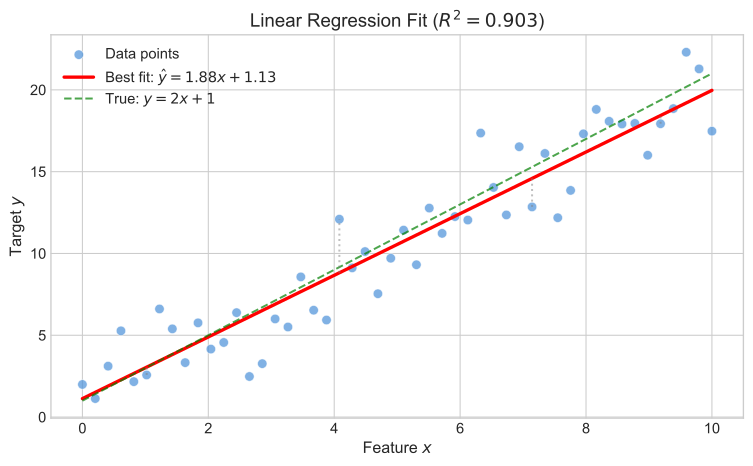
Core Formulation

Model

$$\hat{y}=w_0+w_1{x}_1+w_2{x}_2+\cdots +w_n{x}_n={\mathbf{w}}^T\mathbf{x}+b$$

Matrix form: $\hat{\mathbf{y}}=\mathbf{X}\mathbf{w}$

Loss Function (Mean Squared Error)

$$\mathcal{L}(\mathbf{w})=\frac{1}{n}\sum _{i=1}^n(y_i-{\hat{y}}_i{)}^2=\frac{1}{n}\parallel \mathbf{y}-\mathbf{X}\mathbf{w}{\parallel }^2$$

Goal

Find weights $\mathbf{w}$ that minimize MSE.

---

Solution Methods

Method 1: Normal Equation (Closed-Form)

$$\mathbf{w}=({\mathbf{X}}^T\mathbf{X}{)}^{-1}{\mathbf{X}}^T\mathbf{y}$$

Derivation:

1. Take derivative: $\frac{\partial \mathcal{L}}{\partial \mathbf{w}}=-\frac{2}{n}{\mathbf{X}}^T(\mathbf{y}-\mathbf{X}\mathbf{w})$
2. Set to zero and solve: ${\mathbf{X}}^T\mathbf{y}={\mathbf{X}}^T\mathbf{X}\mathbf{w}$
3. Result: $\mathbf{w}=({\mathbf{X}}^T\mathbf{X}{)}^{-1}{\mathbf{X}}^T\mathbf{y}$

Aspect	Details
When to use	$d<\mathrm{10,000}$ features, ${\mathbf{X}}^T\mathbf{X}$ invertible
Time complexity	$O(n{d}^2+d^3)$
Space complexity	$O(d^2)$

Method 2: Gradient Descent

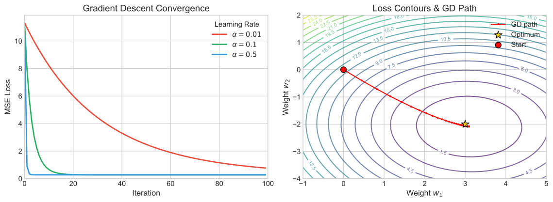
Update rule: $\mathbf{w}\leftarrow \mathbf{w}-\alpha {\mathrm{\nabla }}_{\mathbf{w}}\mathcal{L}$

Gradient: ${\mathrm{\nabla }}_{\mathbf{w}}\mathcal{L}=\frac{2}{n}{\mathbf{X}}^T(\mathbf{X}\mathbf{w}-\mathbf{y})$

def gradient_descent_linear(X, y, lr=0.01, n_iters=1000):
    n, d = X.shape
    w = np.zeros(d)
    for _ in range(n_iters):
        predictions = X @ w
        gradient = (2/n) * X.T @ (predictions - y)
        w = w - lr * gradient
    return w

Aspect	Details
When to use	Large $d$, online learning, with regularization
Time complexity	$O(nd)$ per iteration

---

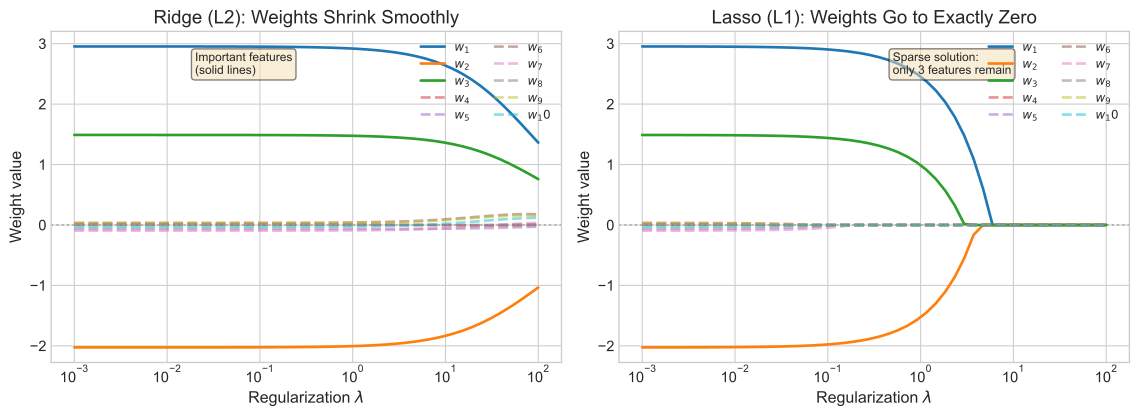
Regularization

Method	Loss Function	Effect	Closed-Form
Ridge (L2)	$|\mathbf{y}-\mathbf{X}\mathbf{w}{|}^2+\lambda |\mathbf{w}{|}_2^2$	Shrinks weights toward zero	$\mathbf{w}=({\mathbf{X}}^T\mathbf{X}+\lambda \mathbf{I}{)}^{-1}{\mathbf{X}}^T\mathbf{y}$
Lasso (L1)	$|\mathbf{y}-\mathbf{X}\mathbf{w}{|}^2+\lambda |\mathbf{w}{|}_1$	Drives weights to exactly zero	No (use coordinate descent)
Elastic Net	$|\mathbf{y}-\mathbf{X}\mathbf{w}{|}^2+{\lambda }_1|\mathbf{w}{|}_1+{\lambda }_2|\mathbf{w}{|}_2^2$	Combines sparsity + stability	No

---

Assumptions

Assumption	Meaning	Check	If Violated
Linearity	$y$ is linear in $\mathbf{x}$	Residual vs. fitted plot	Add polynomial features
Independence	Errors are independent	Durbin-Watson test	Time-series models
Homoscedasticity	Constant error variance	Residuals vs. fitted	Weighted least squares
Normality	$ϵ\sim \mathcal{N}(0,{\sigma }^2)$	Q-Q plot	Less critical for large $n$
No multicollinearity	Features not highly correlated	VIF > 10 is concerning	Remove features or regularize

---

Interpretation

Coefficient Meaning

• Standardized features: "A 1 std increase in $x_j$ $\to$ $w_j$ std change in $y$"
• Raw features: "A 1 unit increase in $x_j$ $\to$ $w_j$ unit change in $y$"

$R^2$ (Coefficient of Determination)

$$R^2=1-\frac{S{S}_{res}}{S{S}_{tot}}=1-\frac{\sum (y_i-{\hat{y}}_i{)}^2}{\sum (y_i-\overline{y}{)}^2}$$

Value	Interpretation
$R^2=1$	Perfect fit
$R^2=0$	No better than mean
$R^2<0$	Worse than mean

Adjusted $R^2$ penalizes adding features:

$$R_{adj}^2=1-(1-R^2)\frac{n-1}{n-d-1}$$

---

Interview Questions

Q1: When use linear regression over complex models?

• Interpretability needed - stakeholders must understand contributions
• Approximately linear relationship - or can engineer features
• Limited data - complex models overfit
• Baseline model - always start simple

Q2: L1 vs L2 regularization?

L1 (Lasso)	L2 (Ridge)
Drives weights to exactly zero	Shrinks but keeps all features
Feature selection	Handles correlated features better
Sparse models	More stable coefficients

If unsure: Use Elastic Net (combines both) with cross-validation.

Q3: What does multicollinearity do?

• Effect: Coefficients unstable, uninterpretable (high variance)
• Detection: Correlation matrix, VIF > 10
• Fix: Remove correlated features, combine them, or use regularization

Q4: Non-linear relationships?

1. Feature engineering - polynomial ($x^2$, $x^3$), interactions ($x_1\cdot x_2$), log transforms
2. Splines - piecewise polynomial fitting
3. Non-linear models - trees, neural networks

---

Code Reference

import numpy as np

class LinearRegression:
    def __init__(self, method='normal', lr=0.01, n_iters=1000,
                 regularization=None, lambda_=0.1):
        self.method = method
        self.lr = lr
        self.n_iters = n_iters
        self.regularization = regularization
        self.lambda_ = lambda_
        self.weights = None

    def fit(self, X, y):
        X = np.c_[np.ones(len(X)), X]  # Add bias

        if self.method == 'normal':
            if self.regularization == 'l2':
                I = np.eye(X.shape[1])
                I[0, 0] = 0  # Don't regularize bias
                self.weights = np.linalg.inv(X.T @ X + self.lambda_ * I) @ X.T @ y
            else:
                self.weights = np.linalg.inv(X.T @ X) @ X.T @ y
        else:  # Gradient descent
            self.weights = np.zeros(X.shape[1])
            for _ in range(self.n_iters):
                grad = (2/len(X)) * X.T @ (X @ self.weights - y)
                if self.regularization == 'l2':
                    grad[1:] += 2 * self.lambda_ * self.weights[1:]
                self.weights -= self.lr * grad

    def predict(self, X):
        X = np.c_[np.ones(len(X)), X]
        return X @ self.weights

    def score(self, X, y):
        """R^2 score"""
        y_pred = self.predict(X)
        ss_res = np.sum((y - y_pred) ** 2)
        ss_tot = np.sum((y - np.mean(y)) ** 2)
        return 1 - ss_res / ss_tot

---

Quick Reference Card

LINEAR REGRESSION
-------------------------------------------------
Model:    y_hat = Xw
Loss:     MSE = (1/n)||y - Xw||^2
Solution: w = (X'X)^{-1}X'y  OR  gradient descent

REGULARIZATION
-------------------------------------------------
L2 (Ridge): + lambda||w||^2  -> shrinks weights
L1 (Lasso): + lambda|w|      -> sparse weights

ASSUMPTIONS
-------------------------------------------------
1. Linearity
2. Independence of errors
3. Homoscedasticity (constant variance)
4. Normality of errors
5. No multicollinearity

COMPLEXITY
-------------------------------------------------
Normal equation: O(nd^2 + d^3) time, O(d^2) space
Gradient descent: O(nd) per iteration

USE WHEN
-------------------------------------------------
- Interpretability needed
- Linear relationship (or engineerable)
- Baseline model
- Small-medium dataset