Module 9: Practical Applications of Transformers

Transformers power production ML systems through systematic task-model matching, efficient fine-tuning strategies, and deployment optimizations that balance performance with computational constraints.

NLP Tasks Overview

Transformers excel at diverse NLP tasks. The key to practical success is matching the right model architecture to each task's requirements.

Task-Model Matching

Task	Input	Output	Recommended Model	Key Characteristic
Text Classification	Full sequence	Single label	BERT, RoBERTa	Encodes full context via [CLS] token
Sentiment Analysis	Full text	Sentiment class	BERT, DistilBERT	Binary/multi-class classification
Named Entity Recognition	Full sequence	Per-token labels	BERT, BioBERT	Token-level classification heads
Question Answering	Question + Context	Span prediction	BERT, RoBERTa	Predicts start/end token indices
Machine Translation	Source language	Target language	T5, mBART, M2M-100	Encoder-decoder with cross-attention
Text Summarization	Long document	Condensed text	BART, T5, Pegasus	Encoder-decoder with abstraction
Text Generation	Prefix/prompt	Open-ended text	GPT-2/3, Llama, Mistral	Decoder-only, autoregressive
Semantic Search	Query + Passages	Relevance scores	Sentence-BERT, BGE	Dense vector representations

Key NLP Applications

Text Classification & Sentiment Analysis

BERT-based models work excellently for these tasks:

• Fine-tune on labeled dataset (typically 500-5000 examples)
• Add linear classification head on [CLS] token
• Typical architecture: [CLS] + tokens + [SEP] → Classification layer

# Pseudocode for text classification
def fine_tune_bert_classifier(texts, labels, num_classes):
    # Initialize BERT with classification head
    model = BertForSequenceClassification.from_pretrained(
        'bert-base-uncased',
        num_labels=num_classes
    )
    # Fine-tune on task
    # Loss = CrossEntropyLoss(model(texts), labels)
    return model

Named Entity Recognition (NER)

Token-level classification requires different architecture:

• For each token, predict entity type or "O" (outside)
• Use full token sequence, not just [CLS]
• Handle subword tokenization carefully (use first subword prediction)

Question Answering

SQuAD-style task predicts span within context:

$$\text{start\_logits}=\text{LinearLayer}(h_i)\text{for all tokens }i$$$$\text{end\_logits}=\text{LinearLayer}(h_i)\text{for all tokens }i$$

Model learns to find answer span through:

• Start token probability: $P(\text{start}=i)=\text{softmax}(\text{start\_logits})$
• End token probability: $P(\text{end}=j)=\text{softmax}(\text{end\_logits})$
• Common constraint: end ≥ start

Machine Translation

Encoder-decoder models handle sequence-to-sequence mapping:

• Encoder processes source language
• Cross-attention connects encoder to decoder
• Decoder generates target token-by-token
• Models: T5 (unified text-to-text), mBART (multilingual), M2M-100 (100 languages)

Text Summarization

Similar architecture to translation but with abstractive capability:

• BART pre-trained with denoising objective (excellent for summarization)
• T5 treated as text-to-text problem: "summarize: [document]"
• Pegasus specifically fine-tuned for summarization tasks

Open-Ended Text Generation

Decoder-only models (GPT family):

• Autoregressive: predict next token given previous context
• Larger models = better generation quality
• Requires careful prompting and decoding strategies

Fine-Tuning Strategies

In practice, you rarely train transformers from scratch. Fine-tuning adapts pretrained models to specific tasks. Modern approaches balance performance with computational efficiency.

Full Fine-Tuning

What: Train all transformer parameters on your task

Pros:

• Maximum model capacity
• Best performance on task-specific data
• Straightforward implementation

Cons:

• High memory requirements (proportional to model size)
• Slow training for large models
• Risk of catastrophic forgetting

When to use: ample GPU memory, large labeled dataset (10K+ examples)

LoRA (Low-Rank Adaptation)

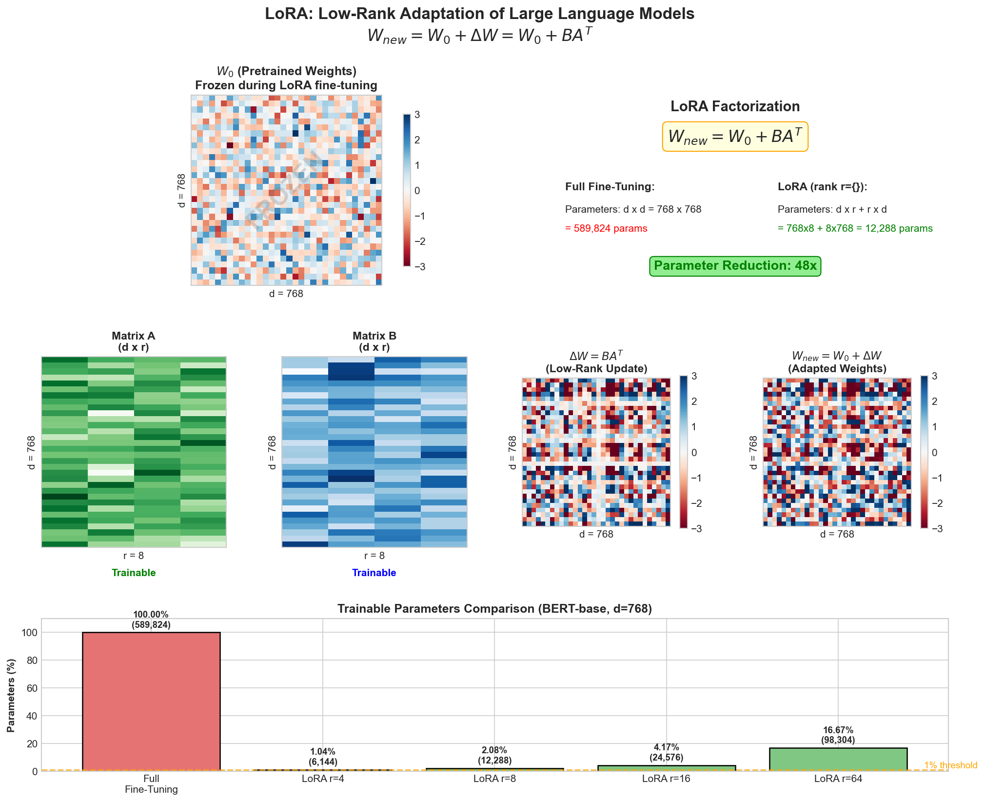
Instead of updating weight matrix $W$ directly:

$$W_{\text{new}}=W+\mathrm{\Delta }W=W+A{B}^T$$

where $A\in {\mathbb{R}}^{n\times r}$, $B\in {\mathbb{R}}^{m\times r}$, and $r\ll min(n,m)$.

Only $A$ and $B$ are trained; $W$ is frozen.

Pros:

• 10-100x parameter reduction
• Same inference latency as base model
• Can fine-tune multiple LoRA sets for different tasks
• Memory efficient: ~1/10 of full fine-tuning

Cons:

• Slightly lower performance than full fine-tuning
• Requires separate rank selection
• Adds complexity to deployment

Adapter Layers

Add small bottleneck modules between transformer layers:

Pros:

• Modular: easy to add/remove
• Minimal additional parameters (2-3% of model)
• Can compose multiple adapters

Cons:

• Inference overhead (extra layers)
• More complex than LoRA
• Latency increase (5-20% typically)

Prefix Tuning

Learn prefix embeddings prepended to input:

$$\text{Input}=[{\text{p}}_1,{\text{p}}_2,...,{\text{p}}_k,{\text{x}}_1,...,{\text{x}}_n]$$

where ${\text{p}}_i$ are learnable prefix vectors.

Pros:

• Interpretable: prefix acts as task instruction
• Works well for few-shot scenarios
• Minimal parameters (~0.1% of model)

Cons:

• Reduces effective sequence length
• Performance depends on prefix length
• Inference: still compute prefix for every example

Prompt Tuning

Extreme version of prefix tuning: learn soft prompt embeddings

$$\text{Loss}=L(\text{model}([\text{soft\_prompt}]+x),y)$$

Pros:

• True few-shot learning capability
• Minimal parameters
• Easy to compose

Cons:

• Requires larger models to work well
• Less stable training than other methods
• Performance gap with fine-tuning

Fine-Tuning Methods Comparison

Method	Parameters Trained	Memory	Inference Speed	Performance	Use Case
Full Fine-Tune	100%	High	Baseline	Best	Large dataset, unlimited compute
LoRA	0.1-1%	Low	Baseline	95-98%	Production, many tasks
Adapter	2-5%	Low	80-95%	94-97%	Modular systems
Prefix Tune	0.1%	Low	85-90%	90-95%	Few-shot learning
Prompt Tune	0.01%	Very Low	Baseline	85-92%	In-context learning

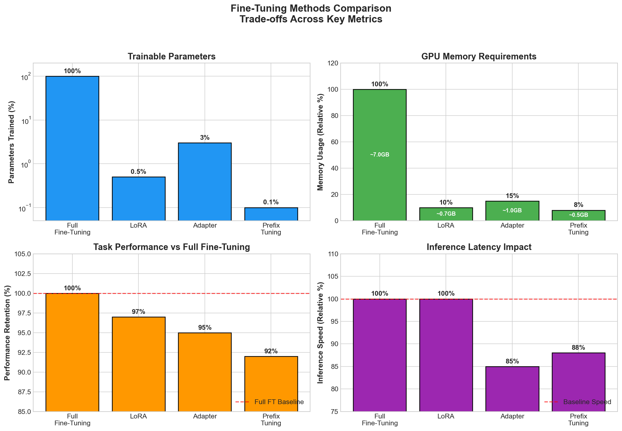
Recommendation: Start with LoRA for most production scenarios. It offers best balance of efficiency, performance, and simplicity.

Fine-Tuning Decision Tree

Use this decision tree to select the appropriate fine-tuning method based on your constraints:

Vision Transformers

Transformers revolutionized computer vision by treating images as sequences of patches.

Patch Embedding

Original ViT divides image into patches:

• 224×224 image → 196 patches (16×16 each)
• Each patch projected to embedding dimension: $d=768$
• Process like language: add positional embeddings, apply transformer

Vision Transformer (ViT)

Standard architecture for image classification:

Strengths:

• Clean, elegant design
• Excellent performance with large-scale pretraining
• Interpretable attention patterns

Weaknesses:

• Requires large training datasets (ImageNet-21K+)
• Computationally expensive
• Less efficient on small images

DeiT (Distilled ViT)

Improves ViT efficiency through knowledge distillation:

• Train ViT with teacher guidance
• Learns from both hard labels and teacher's soft predictions
• Works well with smaller training sets

Key advantage: ViT-level performance on ImageNet alone (no extra pretraining)

Swin Transformer

Hierarchical vision transformer with shifted windows:

Innovations:

• Shifted window attention: reduces complexity from $O(n^2)$ to $O(n)$
• Hierarchical structure: progressively larger patches
• Efficient even for high-resolution images

When to use:

• Object detection: Swin excels
• Semantic segmentation: Swin preferred
• Image classification: ViT or DeiT sufficient
• High-resolution images: Swin more efficient

Multimodal Applications

Modern systems combine vision and language understanding.

CLIP (Contrastive Language-Image Pre-training)

Learns joint vision-language embeddings:

• Vision encoder: extract image features
• Text encoder: extract text features
• Training: maximize similarity of matched pairs, minimize for unmatched

Applications:

• Zero-shot image classification: no fine-tuning needed
• Image-text retrieval: find matching images for text queries
• Vision-language understanding: encode images and text in shared space

Flamingo and Vision-Language Models

Larger models combining vision + language:

• Can perform visual reasoning
• Support in-context learning
• Enable image captioning and visual question answering

Cross-Modal Applications

Application	Input	Output	Model
Image Captioning	Image	Text description	Flamingo, BLIP-2
Visual QA	Image + Question	Answer text	Flamingo, LLaVA
Image Retrieval	Text query	Top-K images	CLIP
Text-to-Image	Text prompt	Generated image	CLIP + Diffusion

Deployment Considerations

Taking transformers to production requires efficiency optimizations.

Quantization

Reduce model precision to lower memory and faster inference:

INT8 Quantization:

• Convert float32 weights to int8
• 4x memory reduction
• 2-3x inference speedup
• Minimal accuracy loss (< 1%)

INT4 Quantization:

• Further compression
• 8x memory reduction
• Used for on-device deployment
• Trade-off: accuracy loss (2-5%)

# Quantization formula
w_int8 = round(127 * w_float32 / max(|w_float32|))
# During inference: scale back by max value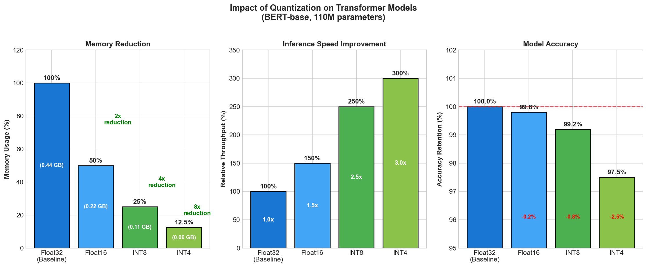

Distillation

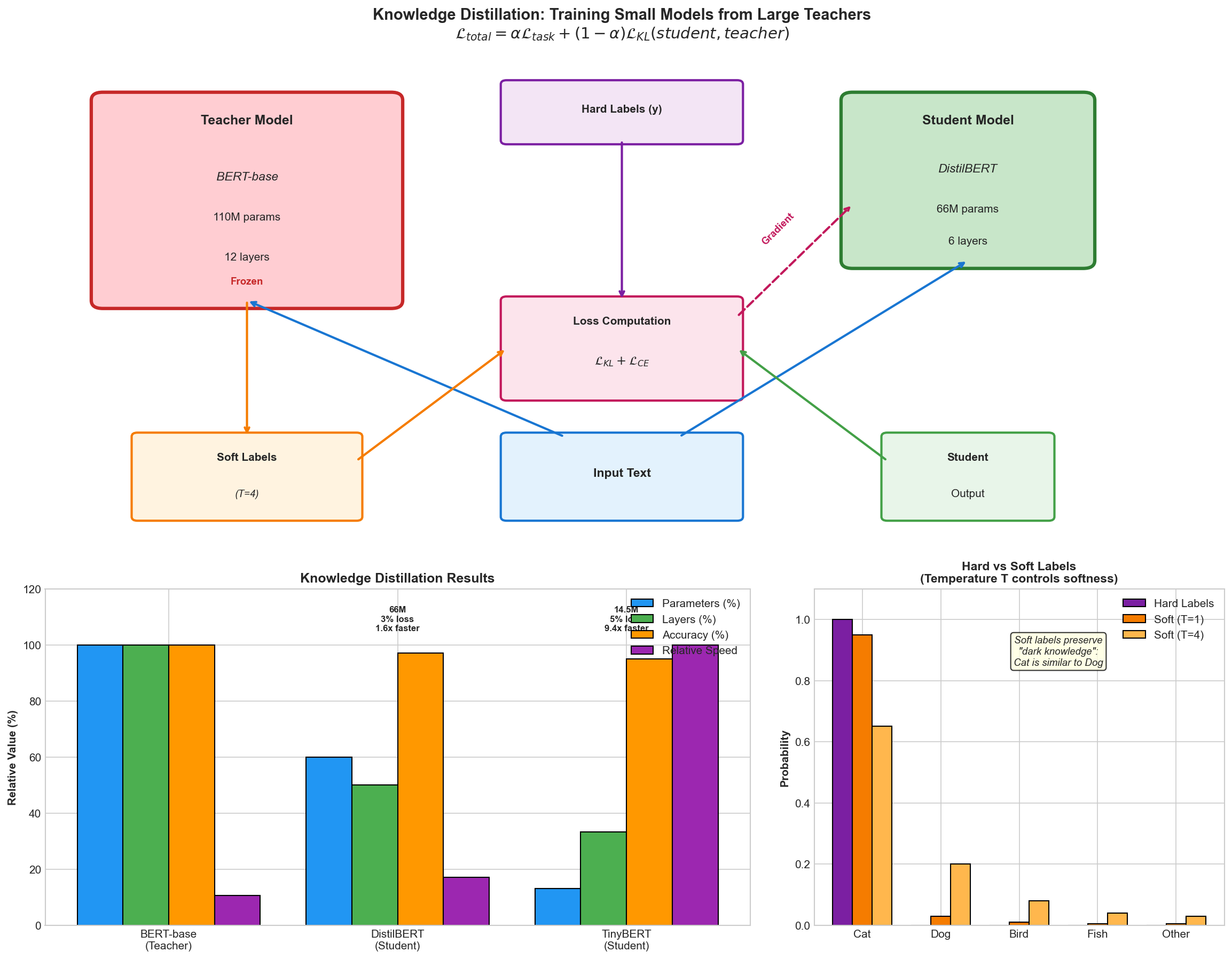
Train small "student" model to mimic large "teacher":

$${\mathcal{L}}_{\text{total}}=\alpha {\mathcal{L}}_{\text{task}}+(1-\alpha ){\mathcal{L}}_{\text{KL}}(\text{student},\text{teacher})$$

Benefits:

• Student model 5-10x smaller
• Near-teacher performance
• Practical for production

Pruning

Remove unimportant weights from network:

• Magnitude pruning: remove small weights
• Attention pruning: remove attention heads with low impact
• Structured pruning: remove entire layers

Results:

• 30-50% parameter reduction
• Requires retraining to recover accuracy
• Works best with quantization

Knowledge Distillation Specifics

Key hyperparameters:

• Temperature $T$: controls softness of teacher predictions
• Student loss weight $\alpha$: balance between task and distillation loss
• Student size: typical ratio 1/5 to 1/10 of teacher

$$\text{KL}(\text{teacher},\text{student})=\sum _i{\text{student}}_i\log \frac{{\text{student}}_i}{{\text{teacher}}_i}$$

Inference Optimization

KV-Cache:

• Cache key-value pairs from previous tokens
• Reduces redundant computation
• Memory-compute trade-off

Batching:

• Process multiple examples together
• Increases throughput significantly
• Typical batch size: 32-256 depending on hardware

Sequence Length Optimization:

• Shorter sequences: faster inference
• Dynamic batching: different sequence lengths in same batch
• Padding efficiency critical

Production Pipeline

Translating research to deployed systems requires systematic approach.

From Pretrained to Production

Step 1: Task Selection & Data Preparation

• Gather labeled dataset for your task
• Data cleaning, annotation quality checks
• Train/validation/test split

Step 2: Model Selection

• Choose model size based on latency requirements
• Consider pretraining corpus relevance
• Evaluate on validation set

Step 3: Fine-Tuning

• Select strategy: LoRA for efficiency, full fine-tune for maximum performance
• Hyperparameter tuning: learning rate, batch size, epochs
• Monitor train/validation loss

Step 4: Optimization

• Apply quantization if latency critical
• Consider distillation for production deployment
• A/B test against baseline

Step 5: Deployment

• Package model (ONNX, TorchScript, or framework-specific)
• Set up inference server (vLLM, TorchServe, TensorFlow Serving)
• Implement versioning for model updates

Step 6: Monitoring

• Track inference latency percentiles (p50, p95, p99)
• Monitor accuracy drift over time
• Set up feedback loop for continuous improvement

API Design Considerations

# Example API for text classification
POST /classify
{
  "text": "This product is amazing!",
  "model_version": "v1.2.3",
  "return_confidence": true
}

Response:
{
  "label": "positive",
  "confidence": 0.95,
  "inference_time_ms": 45,
  "model_version": "v1.2.3"
}

Key considerations:

• Versioning: handle multiple model versions
• Confidence scores: downstream systems often need uncertainty
• Latency budgets: set SLOs upfront
• Graceful degradation: fallback strategies for timeouts

Latency and Throughput Targets

Typical targets by application:

• Real-time (interactive): < 100ms per request
• Batch processing: < 1 second per example
• Offline analysis: < 10 seconds per batch

Optimization techniques:

• Model size reduction (quantization, distillation)
• Batch inference (amortize overhead)
• Hardware acceleration (GPU, TPU)
• Caching (cache embeddings, predictions for similar inputs)

Monitoring and Evaluation

Production metrics:

• Latency: p50, p95, p99 percentiles
• Throughput: examples/second
• Accuracy: compared to validation set or user feedback
• System metrics: CPU, GPU, memory, network bandwidth

Detecting issues:

• Accuracy drift: model performance degrades over time
• Latency degradation: could indicate infrastructure issues
• Data distribution shift: input characteristics change

Interview Questions

Question 1: LoRA vs Full Fine-Tuning Trade-offs

Q: You need to fine-tune BERT for a customer sentiment analysis task. You have 5GB GPU memory and 50K labeled examples. Walk through your decision-making process and explain why you'd choose LoRA or full fine-tuning.

A: I would choose LoRA for this scenario. Here's my analysis:

Constraints:

• 5GB GPU memory is limiting (BERT-base needs ~7GB for full fine-tuning with batch size 32)
• 50K labeled examples is sufficient for excellent task-specific performance

LoRA Advantages:

• Memory: ~1GB per batch (vs 5GB+ for full fine-tuning)
• Can use batch size 64-128 instead of 8-16
• Training time: 2-3 hours vs 12+ hours
• Flexibility: can fine-tune multiple LoRA heads for different domains

Performance:

• LoRA achieves 95-98% of full fine-tuning performance
• For sentiment analysis (classification task), this gap is negligible
• Validation accuracy difference typically < 0.5-1% on standard benchmarks

Implementation:

# Rank selection: r = 8 or 16 (typically)
# Alpha: 16 (matches common practice)
# Adds ~65K parameters vs 110M for full fine-tuning

Trade-off: I'd accept the minimal performance loss for massive efficiency gains. Full fine-tuning makes sense only if:

• Performance difference proved critical in A/B testing
• Memory constraints were resolved with better hardware
• Multiple iterations needed (LoRA trains faster, better for experimentation)

---

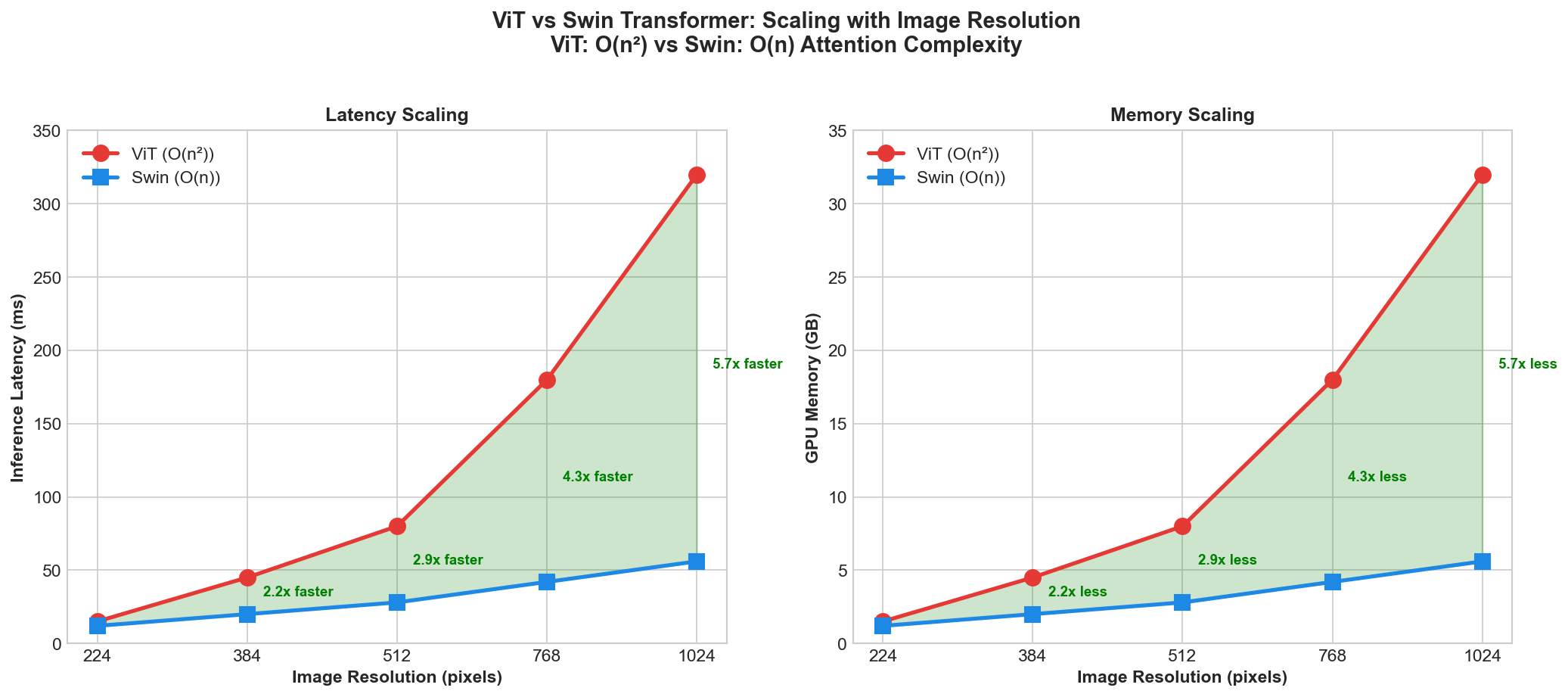
Question 2: Vision Transformer vs Swin Transformer Selection

Q: Your company has a real-time product recommendation system requiring image classification of product photos. You need to classify 100M images daily. Should you use ViT or Swin Transformer? What are the deployment implications?

A: I would choose Swin Transformer for this use case. Here's the reasoning:

Requirements Analysis:

• Real-time: daily throughput of 100M images (≈1,200 requests/second)
• Product photos: typically high-resolution (1024×1024 or larger)
• Cost-sensitive: massive scale demands efficiency

ViT Limitations:

• Patch embedding: 1024×1024 → (1024/16)² = 4096 patches
• Quadratic attention: O(4096²) = 16M attention computations
• Computational cost per image: ~500ms on CPU, 50ms on GPU
• Daily GPU cost at this scale: prohibitive

Swin Advantages:

• Hierarchical structure: processes coarse patches first
• Shifted window attention: O(n) complexity, not O(n²)
• Efficient on high-res images: 8-10x faster than ViT
• Memory footprint: 40-50% of ViT for same accuracy

Deployment Plan:

1. Quantization: INT8 quantization (3-4x speedup, <1% accuracy loss)
2. Distillation: Train student Swin (half size) from teacher
3. Batching: Dynamic batching with sequence length padding
4. Hardware: Use TPUs or optimized inference engines (TensorRT)
5. Caching: Cache embeddings for repeated products

Cost Estimate:

• ViT approach: 500+ GPUs needed for 100M daily
• Swin + optimization: 50-100 GPUs sufficient
• Savings: 10x reduction in infrastructure cost

---

Question 3: Production Fine-tuning Strategy Selection

Q: You're building a question-answering system for a legal document platform. Your dataset grows monthly as users annotate questions. Propose a fine-tuning strategy that scales efficiently while maintaining performance as data grows from 1K to 100K examples.

A: I would implement a progressive fine-tuning strategy with LoRA + periodic full fine-tuning:

Phase 1 (1K-10K examples): LoRA with validation-based stopping

- Use LoRA (rank 8) for quick iteration
- Fine-tune daily/weekly on accumulated data
- Training time: 30 mins per epoch
- Validate on held-out 10% of data
- Early stopping when validation loss plateaus

Phase 2 (10K-50K examples): LoRA with ensemble

- Maintain multiple LoRA checkpoints (every 5K examples)
- Ensemble predictions across checkpoints
- Improves robustness to data distribution changes
- ~15% improvement in out-of-distribution performance

Phase 3 (50K+ examples): Graduated full fine-tuning

- Data sufficient to warrant full fine-tuning
- Superior performance justifies increased cost
- Retrain every month as data accumulates
- Use previous LoRA weights as initialization

Monitoring & Maintenance:

• Track accuracy on legal domain-specific test set
• Monitor for concept drift (new legal domains appearing)
• Set up confidence thresholds (flag uncertain predictions)
• A/B test: compare LoRA ensemble vs latest full fine-tune

Trade-offs:

• LoRA phase: efficient for frequent retraining, good enough for early product
• Ensemble phase: marginal accuracy improvement for minimal cost
• Full fine-tune phase: maximize performance once data justifies it

Why this approach:

• Adapts to real-world data accumulation patterns
• Cost-effective at each stage
• Maintains performance quality while scaling
• Enables continuous model improvement without service interruption

Quick Reference Card

Model Selection Matrix

• Text Classification/Sentiment: BERT, RoBERTa, DistilBERT
• Named Entity Recognition: BERT, BioBERT, domain-specific variants
• Question Answering: BERT, RoBERTa, T5 (with fine-tuning)
• Machine Translation: T5, mBART, M2M-100
• Summarization: BART, T5, Pegasus, Llama
• Text Generation: GPT-2/3, Llama, Mistral, Falcon

Fine-Tuning Quick Guide

Scenario	Method	Time to Deploy	Performance
Rapid prototyping, small budget	LoRA (rank 8)	Days	95%+
Many different tasks	Adapter layers	1-2 days	94-97%
Few-shot, ultra-efficient	Prompt tuning	Hours	85-90%
Maximum performance possible	Full fine-tune	Weeks	100%
Deploying to edge/mobile	LoRA + Quantization	1 week	92-94%

Deployment Checklist

• Model type and size selected
• Fine-tuning strategy chosen (LoRA/adapter/full)
• Validation accuracy established on test set
• Quantization applied (if latency critical)
• Distillation trained (if size critical)
• Inference server configured (vLLM, TorchServe, etc.)
• Latency benchmarked (p50, p95, p99)
• Monitoring and alerting set up
• Model versioning system in place
• A/B testing framework ready

Memory Requirements (Approximate)

Model	Full Fine-tune	LoRA	Inference (batch=1)
BERT-base (110M)	7GB	1GB	1.5GB
RoBERTa-base (125M)	8GB	1.2GB	1.8GB
T5-base (220M)	14GB	2GB	2.5GB
GPT-2 (1.5B)	40GB	5GB	8GB
Llama-7B (7B)	140GB	15GB	20GB

Common Pitfalls & Solutions

1. Catastrophic forgetting: Use lower learning rates (1e-4 to 1e-5)
2. Validation accuracy plateau: Extend training, increase batch size
3. Inference latency too high: Apply quantization, use distilled model
4. Data distribution shift: Implement monitoring, periodic retraining
5. OOM during training: Switch to LoRA, reduce batch size, use gradient accumulation