Model Drift and Monitoring Interview FAQ

Keep models performing well in production

Production ML systems require constant vigilance. Models that perform brilliantly at deployment can silently degrade over time. This FAQ covers the essential concepts for detecting, diagnosing, and addressing model drift in production environments.

---

Fundamental Concepts

Q: What is model drift?

A: Model drift refers to the degradation of a machine learning model's performance over time in production. It occurs when the statistical properties of the data the model encounters differ from the data it was trained on.

Key characteristics:

• Gradual or sudden: Drift can happen slowly over months or abruptly due to external events
• Often invisible: Without proper monitoring, drift goes undetected until business metrics suffer
• Inevitable: In dynamic environments, some degree of drift is expected

Why it matters in interviews: Understanding drift shows you think beyond model training to the full ML lifecycle.

---

Q: What are the main types of drift?

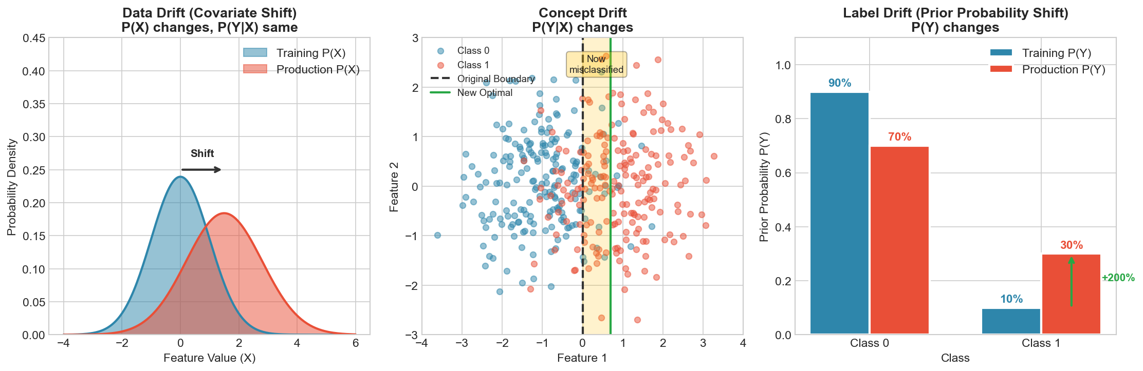
A: There are three primary types of drift, each with distinct causes and detection methods:

Type	What Changes	Detection Method	Example
Data Drift	P(X)	Feature distribution monitoring	User demographics shift
Concept Drift	P(Y|X)	Performance metric degradation	Spam patterns evolve
Label Drift	P(Y)	Target distribution monitoring	Seasonal demand changes

Key insight: Data drift affects what the model sees; concept drift affects how it should respond; label drift affects how often each outcome occurs.

---

Q: What causes model drift?

A: Multiple factors contribute to drift in production systems:

Category	Examples
External	Seasonality, market changes, user behavior evolution, regulatory changes, global events
Internal	Data pipeline issues, feature engineering changes, third-party data source modifications
Adversarial	Users gaming the system, fraud pattern evolution, bot behavior changes

---

Drift Detection Methods

Q: How do you detect data drift using statistical tests?

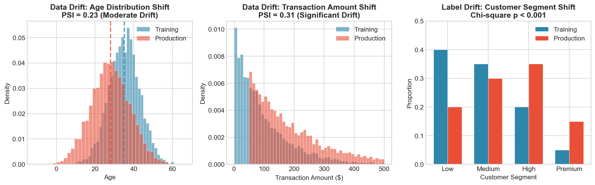
A: Several statistical tests can quantify distribution differences between training and production data:

Test	Best For	Interpretation
KS Test	Continuous features	p-value < 0.05 indicates drift
PSI	Industry standard	< 0.1 stable, 0.1-0.25 moderate, > 0.25 significant
Chi-Square	Categorical features	p-value < 0.05 indicates drift
JS Divergence	Symmetric comparison	0 = identical, 1 = completely different

def calculate_psi(reference, production, bins=10):
    """
    Calculate Population Stability Index.
    PSI < 0.1: No significant shift
    PSI 0.1-0.25: Moderate shift, investigate
    PSI > 0.25: Significant shift, action required
    """
    breakpoints = np.percentile(reference, np.linspace(0, 100, bins + 1))
    breakpoints[0], breakpoints[-1] = -np.inf, np.inf

    ref_props = np.histogram(reference, breakpoints)[0] / len(reference)
    prod_props = np.histogram(production, breakpoints)[0] / len(production)

    ref_props = np.clip(ref_props, 0.0001, None)
    prod_props = np.clip(prod_props, 0.0001, None)

    return np.sum((prod_props - ref_props) * np.log(prod_props / ref_props))

---

Q: How do you detect concept drift?

A: Concept drift requires monitoring model performance, not just input distributions. The decision boundary that was optimal at training time may no longer be optimal:

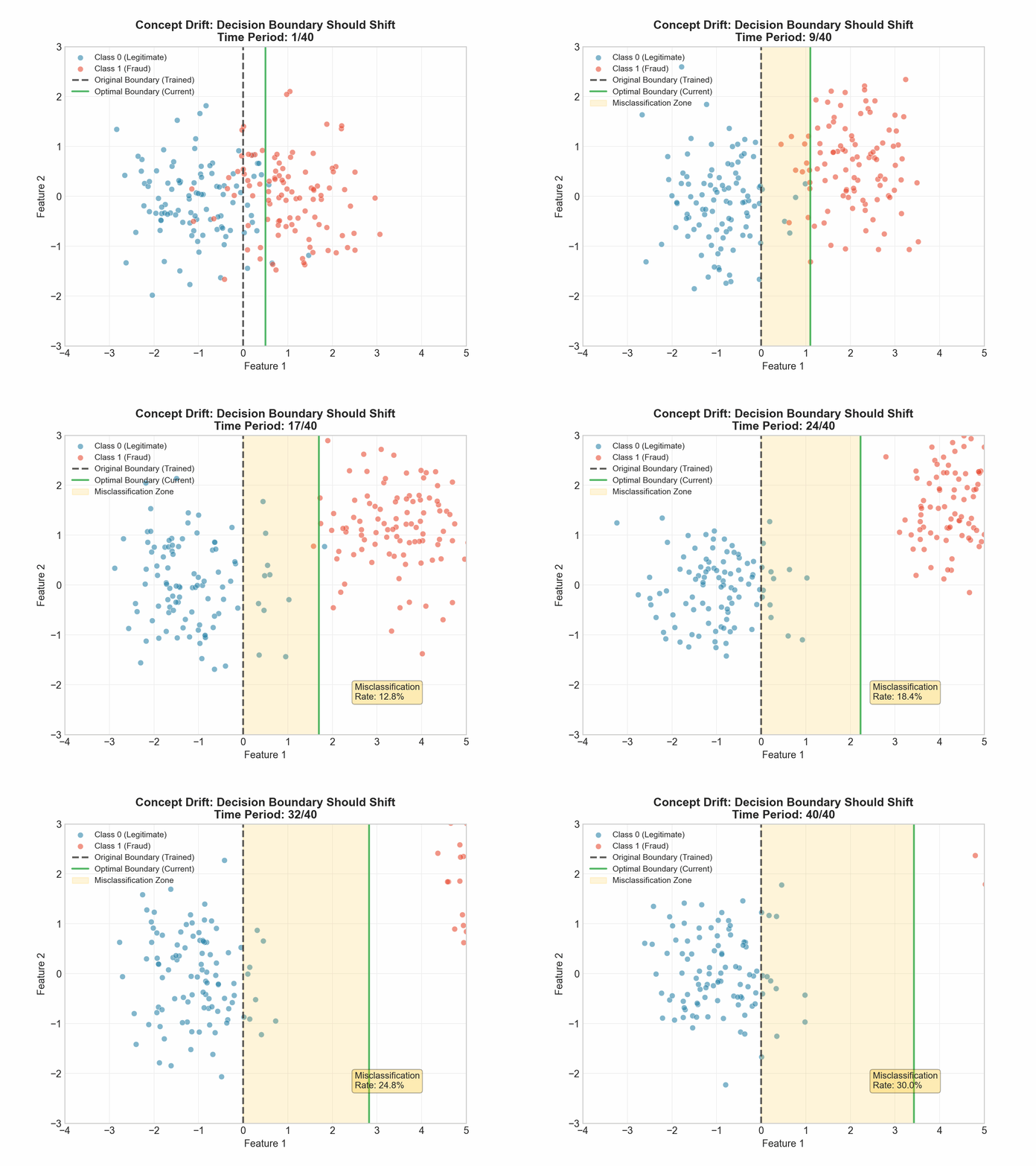
Detection approaches:

Approach	Description	Use Case
Performance-Based	Track accuracy/F1 degradation over time	Labeled feedback available
Sliding Window	Compare metrics across time windows	Detect sudden changes
ADWIN	Adaptive window sizing	Streaming data

def sliding_window_drift_detection(predictions, actuals, window_size=1000):
    """Compare model accuracy across sliding windows."""
    accuracies = []
    for i in range(len(predictions) - window_size):
        accuracy = (predictions[i:i+window_size] == actuals[i:i+window_size]).mean()
        accuracies.append(accuracy)

    baseline_acc = np.mean(accuracies[:100])
    current_acc = np.mean(accuracies[-10:])

    return {
        'baseline_accuracy': baseline_acc,
        'current_accuracy': current_acc,
        'drift_detected': (baseline_acc - current_acc) > 0.05
    }

---

Production Monitoring Strategies

Q: What metrics should you monitor in production ML systems?

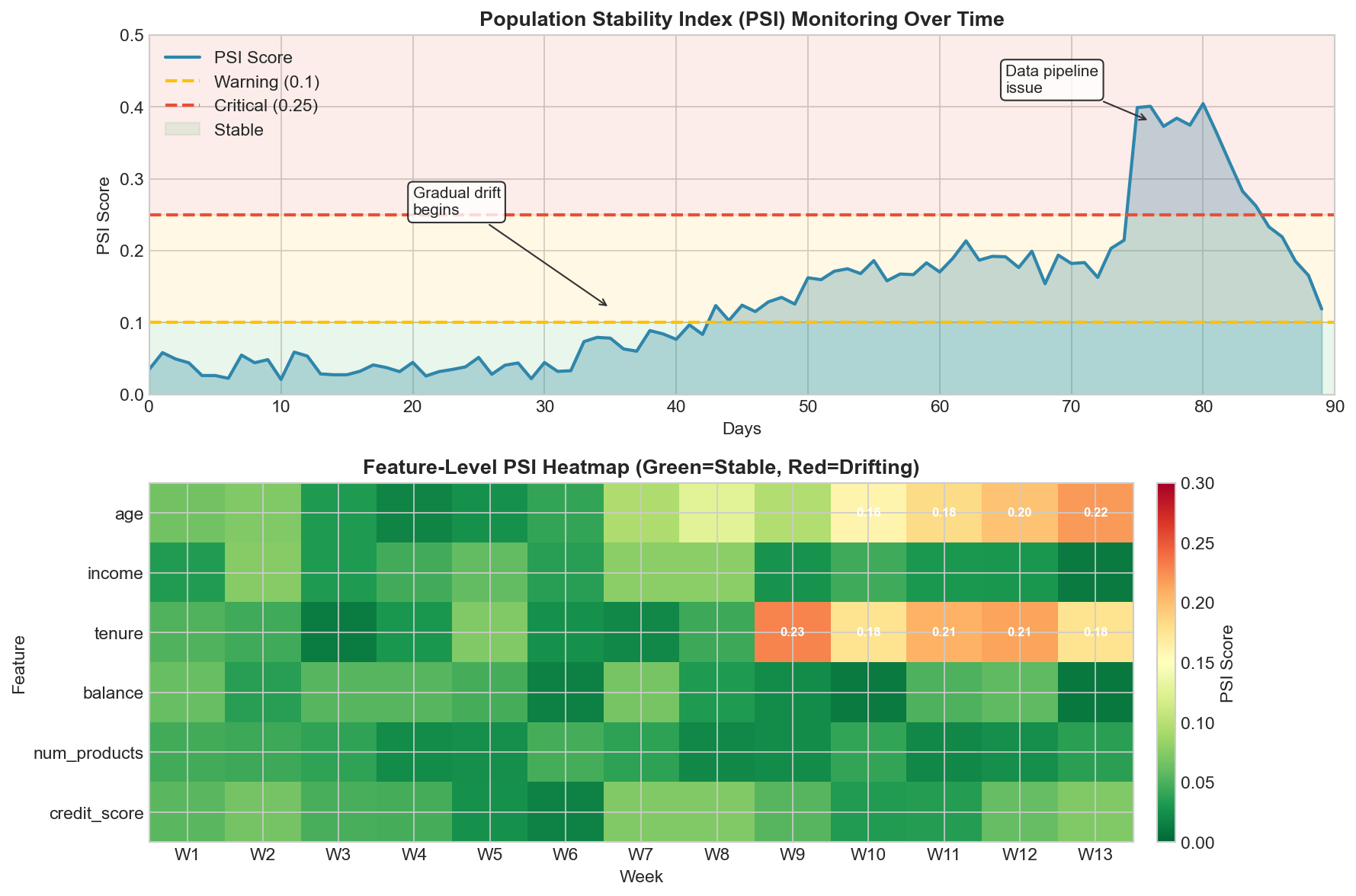
A: A comprehensive monitoring strategy covers multiple layers. Here is a typical monitoring dashboard:

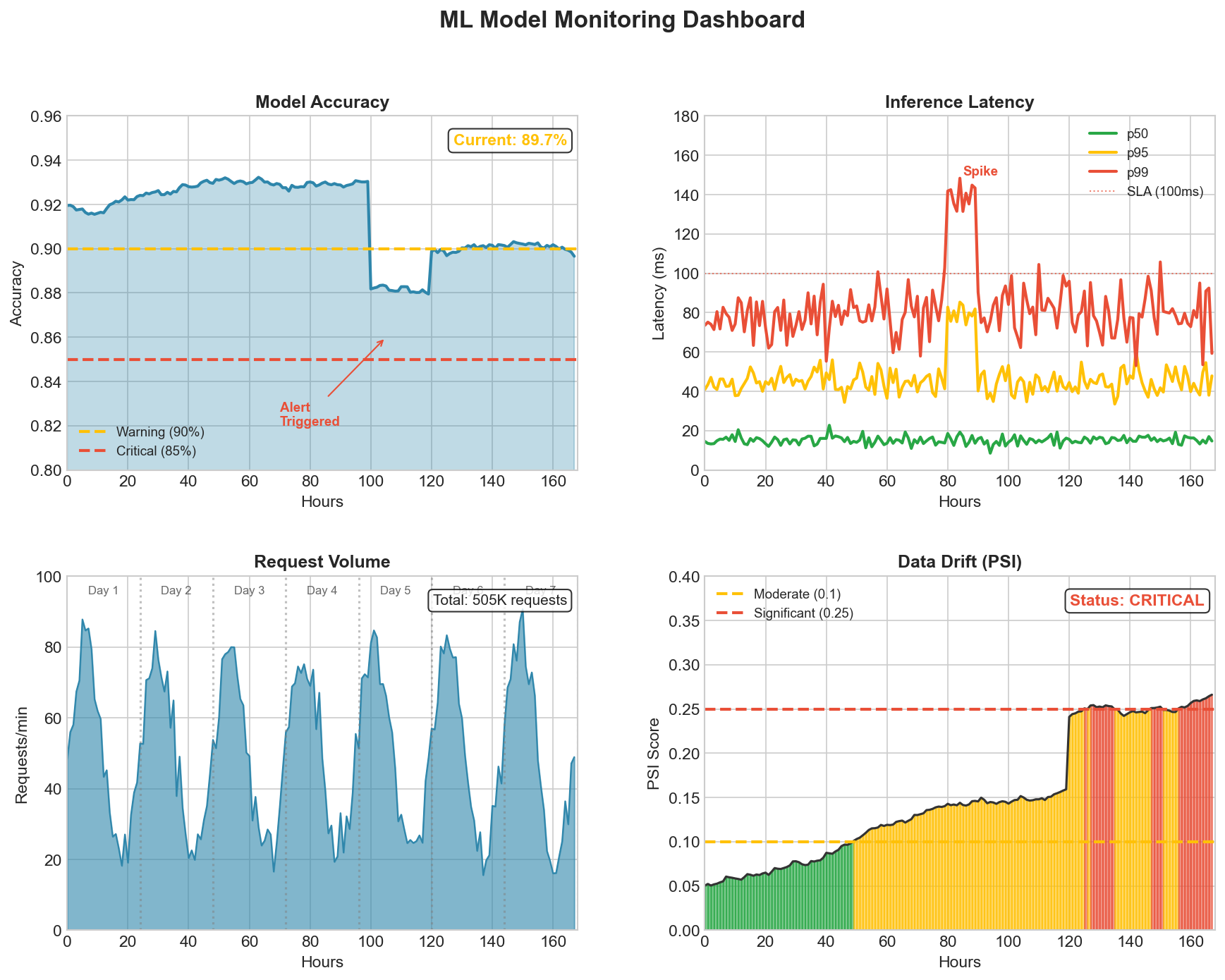
Key metric categories:

Category	Metrics	Alert Thresholds
Performance	Accuracy, Precision, Recall, F1, AUC	> 10% degradation from baseline
Data Quality	Null rates, schema violations, outliers	Any unexpected values
Operational	Latency (p50/p95/p99), throughput, errors	SLA violations
Drift	PSI, KS statistic, JS divergence	PSI > 0.1 warning, > 0.25 critical

---

Q: How do you implement alerting for model drift?

A: Effective alerting requires tiered thresholds and actionable notifications:

Severity	Threshold	Action	Example
Info	< 5% degradation	Log only	Minor fluctuations
Warning	5-15% degradation	Slack notification	Investigate data changes
Critical	> 15% degradation	PagerDuty alert	Consider rollback/retrain

Best practices:

• Set per-metric thresholds based on business impact
• Include recommended actions in alerts
• Track alert patterns to tune thresholds and reduce fatigue

---

Model Retraining Strategies

Q: When should you retrain a model?

A: Retraining decisions should be based on multiple signals:

Trigger Type	Signal	Example Threshold
Performance	Accuracy/F1 degradation	< 90% of baseline
Drift	PSI score	> 0.25
Time	Model age	> 30 days

Retraining strategies:

Strategy	Description	Use Case
Scheduled	Retrain on fixed schedule (daily, weekly)	Stable domains with predictable drift
Triggered	Retrain when metrics cross thresholds	Variable drift patterns
Continuous	Online learning with streaming data	High-velocity environments
Incremental	Fine-tune on new data only	Limited compute resources

---

Deployment Strategies

Q: What is A/B testing for model deployment?

A: A/B testing compares model versions by splitting production traffic:

class ABTestManager:
    """
    Manage A/B tests for model deployment.
    """

    def __init__(self, experiment_config):
        self.control_model = experiment_config['control']
        self.treatment_model = experiment_config['treatment']
        self.traffic_split = experiment_config['traffic_split']  # e.g., 0.5
        self.metrics_to_track = experiment_config['metrics']

    def route_request(self, user_id, request):
        """
        Route request to appropriate model variant.
        Uses consistent hashing for user stickiness.
        """
        # Deterministic assignment based on user_id
        hash_value = hash(user_id) % 100

        if hash_value < self.traffic_split * 100:
            variant = 'treatment'
            prediction = self.treatment_model.predict(request)
        else:
            variant = 'control'
            prediction = self.control_model.predict(request)

        # Log for analysis
        self.log_experiment_event(user_id, variant, prediction)

        return prediction

    def analyze_results(self):
        """
        Statistical analysis of A/B test results.
        """
        control_metrics = self.get_variant_metrics('control')
        treatment_metrics = self.get_variant_metrics('treatment')

        results = {}
        for metric in self.metrics_to_track:
            # Two-sample t-test
            t_stat, p_value = stats.ttest_ind(
                control_metrics[metric],
                treatment_metrics[metric]
            )

            lift = (
                (np.mean(treatment_metrics[metric]) - np.mean(control_metrics[metric]))
                / np.mean(control_metrics[metric])
            ) * 100

            results[metric] = {
                'control_mean': np.mean(control_metrics[metric]),
                'treatment_mean': np.mean(treatment_metrics[metric]),
                'lift_pct': lift,
                'p_value': p_value,
                'significant': p_value < 0.05
            }

        return results

Key considerations:

• Sample size calculation for statistical power
• User-level randomization for consistency
• Guardrail metrics to catch regressions
• Duration based on traffic volume

---

Q: What is shadow deployment?

A: Shadow deployment runs a new model in parallel without affecting users:

class ShadowDeployment:
    """
    Shadow mode deployment for safe model testing.
    """

    def __init__(self, production_model, shadow_model):
        self.production = production_model
        self.shadow = shadow_model
        self.comparison_log = []

    async def predict(self, request):
        """
        Run both models, return production result,
        log shadow result for analysis.
        """
        # Production prediction (returned to user)
        prod_start = time.time()
        prod_result = await self.production.predict(request)
        prod_latency = time.time() - prod_start

        # Shadow prediction (not returned, just logged)
        shadow_start = time.time()
        shadow_result = await self.shadow.predict(request)
        shadow_latency = time.time() - shadow_start

        # Log comparison
        self.comparison_log.append({
            'timestamp': datetime.now(),
            'request_id': request.id,
            'production_result': prod_result,
            'shadow_result': shadow_result,
            'results_match': prod_result == shadow_result,
            'production_latency': prod_latency,
            'shadow_latency': shadow_latency
        })

        return prod_result  # Only production result goes to user

    def analyze_shadow_performance(self):
        """
        Compare shadow model against production.
        """
        df = pd.DataFrame(self.comparison_log)

        return {
            'agreement_rate': df['results_match'].mean(),
            'shadow_avg_latency': df['shadow_latency'].mean(),
            'production_avg_latency': df['production_latency'].mean(),
            'latency_overhead': (
                df['shadow_latency'].mean() / df['production_latency'].mean()
            )
        }

Benefits:

• Zero risk to users
• Real production traffic testing
• Performance comparison under actual load
• Catch issues before any user impact

---

Q: What is canary deployment?

A: Canary deployment gradually rolls out a new model to increasing traffic:

class CanaryDeployment:
    """
    Gradual rollout with automatic rollback.
    """

    def __init__(self, config):
        self.stages = config['stages']  # e.g., [1, 5, 25, 50, 100]
        self.current_stage = 0
        self.success_criteria = config['success_criteria']
        self.rollback_criteria = config['rollback_criteria']

    def execute_rollout(self):
        """
        Execute staged rollout with monitoring.
        """
        for stage_pct in self.stages:
            print(f"Rolling out to {stage_pct}% of traffic...")

            self.set_traffic_percentage(stage_pct)

            # Wait for metrics to stabilize
            time.sleep(self.observation_period)

            # Check health
            metrics = self.collect_stage_metrics()

            if self.should_rollback(metrics):
                print(f"Rollback triggered at {stage_pct}%")
                self.rollback()
                return {'success': False, 'stage': stage_pct}

            if not self.meets_success_criteria(metrics):
                print(f"Pausing at {stage_pct}%, criteria not met")
                continue

            print(f"Stage {stage_pct}% successful")

        return {'success': True, 'stage': 100}

    def should_rollback(self, metrics):
        """
        Check if rollback is needed.
        """
        for metric, threshold in self.rollback_criteria.items():
            if metrics[metric] > threshold:
                return True
        return False

    def rollback(self):
        """
        Immediately revert to previous model.
        """
        self.set_traffic_percentage(0)
        self.restore_previous_model()
        self.alert_team("Canary rollback executed")

Typical canary stages:

1. 1% - Initial test with minimal impact
2. 5% - Early validation
3. 25% - Broader testing
4. 50% - Half traffic
5. 100% - Full rollout

---

Logging and Observability

Q: What should you log for ML observability?

A: Comprehensive logging enables debugging and auditing. Track prediction distributions over time to detect drift:

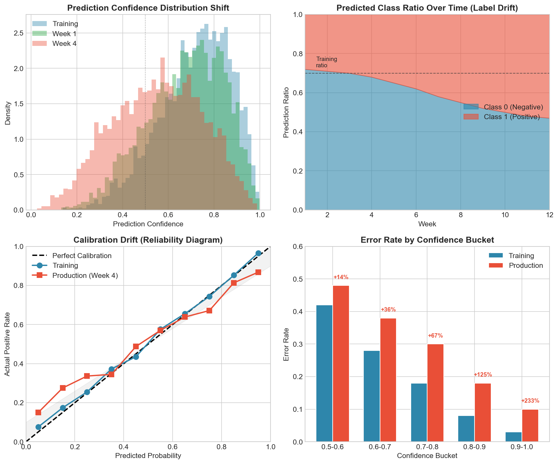
Key logging fields:

Category	Fields
Request	timestamp, request_id, model_version
Features	feature_values (sanitized), feature_hash
Output	prediction, confidence, probabilities
Performance	inference_latency_ms, preprocessing_latency_ms
Context	user_segment, experiment_variant

Key logging principles:

• Structured JSON format for queryability
• Request IDs for tracing
• Feature hashing for privacy
• Separate prediction and outcome logs
• Include model version for debugging

---

Q: How do you build an ML observability dashboard?

A: Essential dashboard components (see monitoring dashboard above):

dashboard_config = {
    'performance_panel': {  # Accuracy, precision, recall over time
        'metrics': ['accuracy', 'precision', 'recall', 'f1', 'auc'],
        'visualization': 'time_series'
    },
    'data_quality_panel': {  # Null rates, schema violations by feature
        'metrics': ['null_rate', 'schema_violations', 'outlier_rate'],
        'visualization': 'heatmap'
    },
    'drift_panel': {  # PSI, KS with threshold lines
        'metrics': ['psi_score', 'ks_statistic', 'js_divergence'],
        'alert_lines': [0.1, 0.25]
    },
    'operational_panel': {
        'metrics': ['latency_p50', 'latency_p99', 'error_rate', 'throughput'],
        'visualization': 'multi_line',
        'sla_lines': True
    },

    'prediction_distribution_panel': {
        'visualization': 'histogram',
        'comparison': 'training_distribution',
        'update_frequency': 'real_time'
    }
}

---

Feature Stores and Data Quality

Q: How do feature stores help with monitoring?

A: Feature stores centralize feature management and enable consistent monitoring:

Capability	Monitoring Benefit
Feature Registry	Track expected types, ranges, allowed values
Version Control	Detect when upstream features change
Statistics Store	Baseline distributions for drift detection
Validation	Automatic checks on retrieval

---

Q: How do you ensure data quality in ML pipelines?

A: Implement validation at multiple pipeline stages:

Check Type	What It Validates	Example
Schema	Expected columns and types	Missing feature, wrong dtype
Completeness	Null rates within bounds	> 5% nulls in required field
Validity	Values within valid ranges	Age < 0 or > 150
Consistency	Cross-field relationships	End date before start date
Freshness	Data recency	Stale data older than 24 hours

---

Interview Tips

Q: How would you design a monitoring system from scratch?

A: Structure your answer around these six layers:

Layer	Components	Tools
1. Data Collection	Prediction logging, ground truth collection, feature statistics	Custom logging
2. Storage	Time-series metrics, feature distributions, logs	InfluxDB, Prometheus, ELK
3. Analysis	Drift detection, performance computation, anomaly detection	Custom + ML libraries
4. Alerting	Threshold, trend, and anomaly-based alerts	PagerDuty, Slack
5. Action	Retraining triggers, rollback, escalation	Airflow, custom pipelines
6. Visualization	Real-time dashboards, historical analysis	Grafana, custom UI

---

Q: What are common pitfalls in production ML monitoring?

A: Be prepared to discuss these challenges:

Pitfall	Description	Mitigation
Delayed ground truth	Labels may take days/weeks to arrive	Use proxy metrics, confidence monitoring
Alert fatigue	Too many false positives	Tune thresholds, aggregate alerts
Metric gaming	Optimizing monitored metrics only	Multiple complementary metrics
Cold start	New models lack baseline	Use holdout set performance
Seasonal patterns	Normal variation mistaken for drift	Seasonal baselines
Multivariate drift	Joint distribution shift	Monitor feature correlations
Feedback loops	Predictions influence future data	Log prediction/outcome separately

class DelayedFeedbackMonitor:
    """Track predictions awaiting ground truth."""

    def log_prediction(self, request_id, prediction, timestamp):
        self.pending[request_id] = {'prediction': prediction, 'timestamp': timestamp}

    def receive_feedback(self, request_id, ground_truth):
        if request_id in self.pending:
            pred_info = self.pending.pop(request_id)
            self.metrics_store.add(pred_info['prediction'], ground_truth)

    def check_missing_feedback(self):
        """Alert on predictions missing expected feedback."""
        overdue = [rid for rid, info in self.pending.items()
                   if (datetime.now() - info['timestamp']).hours > self.expected_delay]
        if len(overdue) > self.threshold:
            self.alert(f"{len(overdue)} predictions missing feedback")

---

Key Takeaways

1. Drift is inevitable - Plan for it from day one
2. Monitor multiple signals - Performance, data quality, and operations
3. Automate responses - Manual monitoring doesn't scale
4. Balance sensitivity - Too many alerts cause fatigue
5. Design for debugging - Good logging pays dividends
6. Test deployment strategies - Shadow, canary, and A/B reduce risk
7. Feature stores help - Centralized management improves consistency
8. Close the feedback loop - Connect predictions to outcomes

Production ML is as much about operations as it is about algorithms. Demonstrating awareness of these challenges shows interview readiness for real-world ML roles.