Value Functions & Bellman Equations

The core mathematics of RL — measuring how good states and actions are

---

State Value Function V(s)

The state value function $V^{\pi }(s)$ measures the expected return starting from state $s$ and following policy $\pi$ thereafter.

$$V^{\pi }(s)={\mathbb{E}}_{\pi }[G_t\mid S_t=s]={\mathbb{E}}_{\pi }[\sum _{k=0}^{\mathrm{\infty }}{\gamma }^k{R}_{t+k+1}\mid S_t=s]$$

Where $G_t$ is the return, $\gamma \in [0,1]$ is the discount factor, and ${\mathbb{E}}_{\pi }$ denotes expectation under policy $\pi$.

Think of $V^{\pi }(s)$ as the "score" of a state—how valuable it is to be there. A state near the goal has high value; a state near a trap has low value.

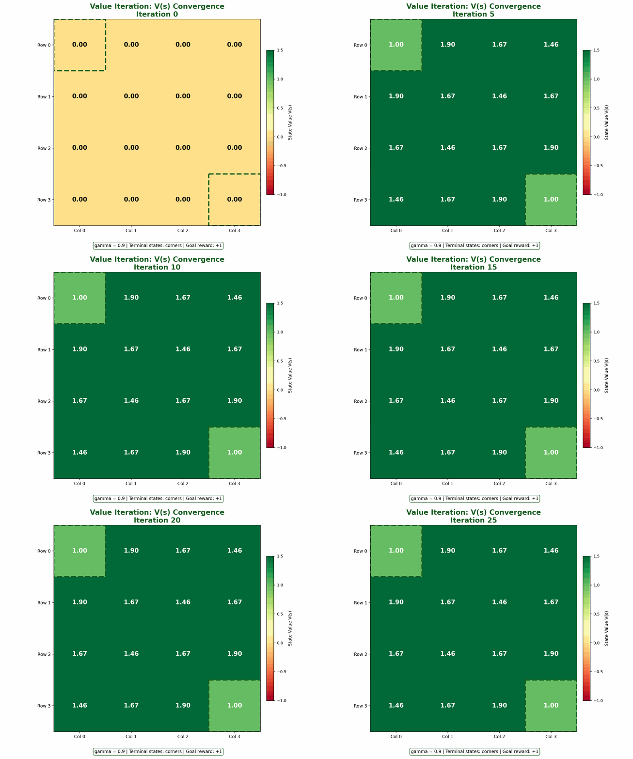
Property	Description
Policy-dependent	Different policies yield different value functions
Bounded	$V^{\pi }(s)\in [\frac{R_{min}}{1-\gamma },\frac{R_{max}}{1-\gamma }]$
Unique	For a fixed policy, there exists a unique value function

---

Action Value Function Q(s, a)

The action value function $Q^{\pi }(s,a)$ measures the expected return starting from state $s$, taking action $a$, and then following policy $\pi$.

$$Q^{\pi }(s,a)={\mathbb{E}}_{\pi }[G_t\mid S_t=s,A_t=a]$$

Q-values allow action selection without a model. Given $Q^{\pi }(s,a)$ for all actions:

$$a^{\ast }=\arg \underset{a}{max}{Q}^{\pi }(s,a)$$

This is why Q-learning and DQN focus on learning Q-values directly.

V and Q Relationship

$$V^{\pi }(s)=\sum _a\pi (a|s)Q^{\pi }(s,a)$$$$Q^{\pi }(s,a)=R(s,a)+\gamma \sum _{s^{\prime }}P(s^{\prime }|s,a)V^{\pi }(s^{\prime })$$

---

Bellman Expectation Equations

The Bellman equations express a recursive relationship: the value of a state depends on successor state values.

Derivation for V(s)

Starting from $V^{\pi }(s)={\mathbb{E}}_{\pi }[G_t\mid S_t=s]$ and expanding the return $G_t=R_{t+1}+\gamma G_{t+1}$:

$$V^{\pi }(s)={\mathbb{E}}_{\pi }[R_{t+1}+\gamma G_{t+1}\mid S_t=s]$$

By linearity and the law of total expectation:

$$V^{\pi }(s)=\sum _a\pi (a|s)\sum _{s^{\prime }}P(s^{\prime }|s,a)[R(s,a,s^{\prime })+\gamma V^{\pi }(s^{\prime })]$$

Bellman Expectation Equation for Q

$$Q^{\pi }(s,a)=\sum _{s^{\prime }}P(s^{\prime }|s,a)[R(s,a,s^{\prime })+\gamma \sum _{a^{\prime }}\pi (a^{\prime }|s^{\prime })Q^{\pi }(s^{\prime },a^{\prime })]$$

Bellman Backup Diagram

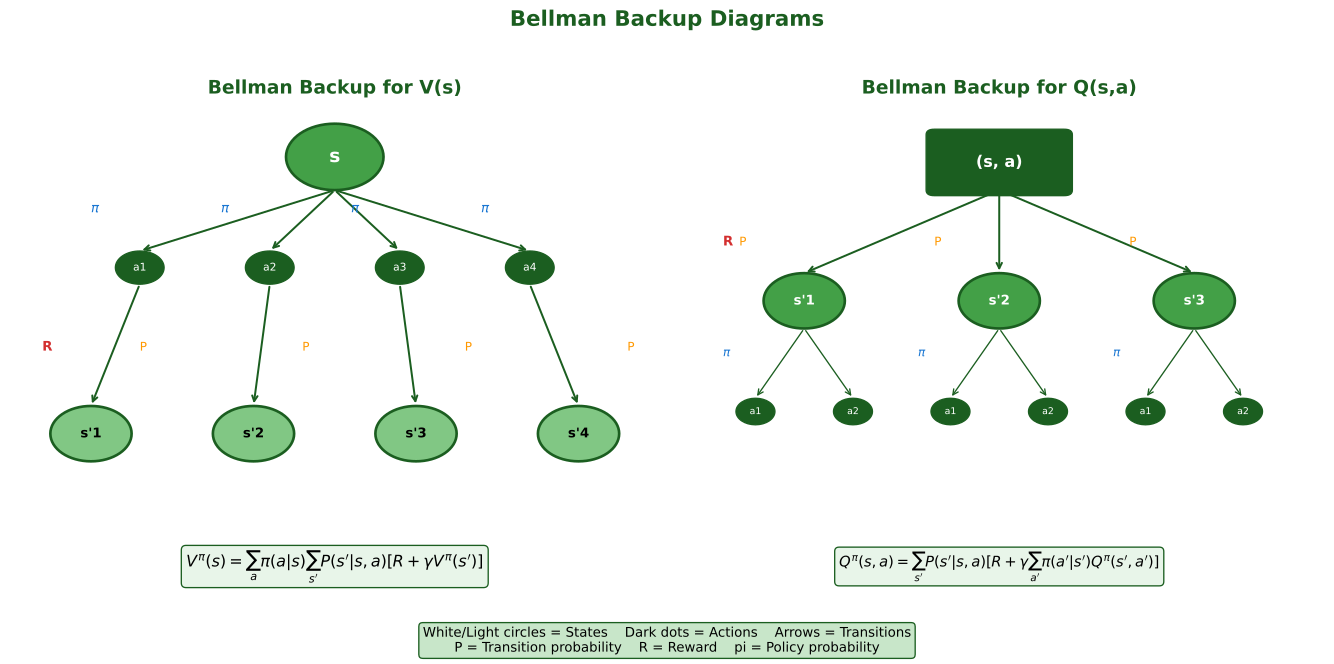
The backup diagram shows how value "flows back" from successor states. White nodes = states; black nodes = state-action pairs.

---

Bellman Optimality Equations

The optimal value functions $V^{\ast }(s)$ and $Q^{\ast }(s,a)$ represent the best possible values achievable by any policy.

$$V^{\ast }(s)=\underset{\pi }{max}{V}^{\pi }(s)=\underset{a}{max}{Q}^{\ast }(s,a)$$

Bellman Optimality for V:*

$$V^{\ast }(s)=\underset{a}{max}\sum _{s^{\prime }}P(s^{\prime }|s,a)[R(s,a,s^{\prime })+\gamma V^{\ast }(s^{\prime })]$$

Bellman Optimality for Q:*

$$Q^{\ast }(s,a)=\sum _{s^{\prime }}P(s^{\prime }|s,a)[R(s,a,s^{\prime })+\gamma \underset{a^{\prime }}{max}{Q}^{\ast }(s^{\prime },a^{\prime })]$$

The key difference from expectation equations: instead of averaging over actions, we take the maximum.

Relationship Between V* and Q*

$$V^{\ast }(s)=\underset{a}{max}{Q}^{\ast }(s,a)\text{and}{Q}^{\ast }(s,a)=R(s,a)+\gamma \sum _{s^{\prime }}P(s^{\prime }|s,a)V^{\ast }(s^{\prime })$$

Once we have $Q^{\ast }$, the optimal policy is: ${\pi }^{\ast }(s)=\arg \underset{a}{max}{Q}^{\ast }(s,a)$

---

Policy Evaluation and Policy Improvement

Policy Evaluation

Compute $V^{\pi }(s)$ by iteratively applying the Bellman expectation equation:

$$V_{k+1}(s)=\sum _a\pi (a|s)\sum _{s^{\prime }}P(s^{\prime }|s,a)[R(s,a,s^{\prime })+\gamma V_k(s^{\prime })]$$

Policy Improvement

Given $V^{\pi }$, construct a better policy by acting greedily:

$${\pi }^{\prime }(s)=\arg \underset{a}{max}\sum _{s^{\prime }}P(s^{\prime }|s,a)[R(s,a,s^{\prime })+\gamma V^{\pi }(s^{\prime })]$$

Policy Improvement Theorem: $Q^{\pi }(s,{\pi }^{\prime }(s))\ge V^{\pi }(s)⟹V^{{\pi }^{\prime }}(s)\ge V^{\pi }(s)$

Policy Iteration

1. Initialize V(s), pi(s) arbitrarily
2. Repeat until policy stable:
   a. Policy Evaluation: Compute V^pi
   b. Policy Improvement: pi' = greedy(V^pi)
   c. If pi' = pi, return (optimal); else pi <- pi'

---

Value Iteration Algorithm

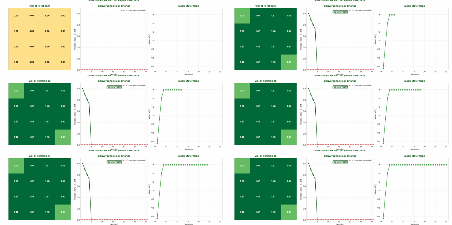
Value iteration combines evaluation and improvement into a single update:

$$V_{k+1}(s)=\underset{a}{max}\sum _{s^{\prime }}P(s^{\prime }|s,a)[R(s,a,s^{\prime })+\gamma V_k(s^{\prime })]$$

Convergence

The Bellman optimality operator is a contraction mapping:

$$\parallel V_{k+1}-V^{\ast }{\parallel }_{\mathrm{\infty }}\le \gamma \parallel V_k-V^{\ast }{\parallel }_{\mathrm{\infty }}$$

Convergence is geometric with rate $\gamma$.

Aspect	Value Iteration	Policy Iteration
Update	Single sweep	Full evaluation
Convergence	Asymptotic	Exact in finite steps
Per-iteration cost	Lower	Higher

---

Summary Comparison

Concept	Formula	Key Insight
$V^{\pi }(s)$	${\mathbb{E}}_{\pi }[G_t\mid S_t=s]$	Expected return from state under policy
$Q^{\pi }(s,a)$	${\mathbb{E}}_{\pi }[G_t\mid S_t=s,A_t=a]$	Expected return from state-action under policy
$V^{\ast }(s)$	$\underset{a}{max}{Q}^{\ast }(s,a)$	Best achievable value from state
$Q^{\ast }(s,a)$	$R+\gamma \underset{a^{\prime }}{max}{Q}^{\ast }(s^{\prime },a^{\prime })$	Best achievable value from state-action
Bellman Expectation	Average over actions	Evaluates a given policy
Bellman Optimality	Max over actions	Finds optimal policy

---

Interview Questions

Q1: When would you prefer learning V(s) vs Q(s,a)?

Answer:

Prefer Q when:

• Model-free learning (unknown transitions)
• Need direct action selection: $a^{\ast }=\arg \underset{a}{max}Q(s,a)$
• Off-policy learning (Q-learning works with any data)

Prefer V when:

• Model is known (derive Q from V cheaply)
• Large action spaces (V has lower memory)
• Actor-Critic methods (critic often estimates V)

Key tradeoff: Q enables model-free action selection but requires $|S|\times |A|$ storage vs $|S|$ for V.

---

Q2: Derive the Bellman equation and explain its computational benefit.

Answer:

From $V^{\pi }(s)={\mathbb{E}}_{\pi }[G_t\mid S_t=s]$, expand $G_t=R_{t+1}+\gamma G_{t+1}$:

$$V^{\pi }(s)=\sum _a\pi (a|s)\sum _{s^{\prime }}P(s^{\prime }|s,a)[R+\gamma V^{\pi }(s^{\prime })]$$

Computational benefit: Instead of simulating infinite trajectories (Monte Carlo), Bellman transforms this into a system of $n$ linear equations solvable in $O(n^3)$ or $O(n^{2}k)$ via iteration. This is dynamic programming.

---

Q3: Why does value iteration converge?

Answer:

The Bellman optimality operator is a contraction: $\parallel TV-T{V}^{\prime }{\parallel }_{\mathrm{\infty }}\le \gamma \parallel V-V^{\prime }{\parallel }_{\mathrm{\infty }}$

By Banach fixed-point theorem, repeated application converges to the unique fixed point $V^{\ast }$.

Convergence rate: Error decreases as ${\gamma }^k$. At $\gamma =0.9$, ~44 iterations for 100x reduction; at $\gamma =0.99$, ~460 iterations.

Stopping criterion: When $\underset{s}{max}|V_{k+1}(s)-V_k(s)|<ϵ$, we have $\parallel V_k-V^{\ast }{\parallel }_{\mathrm{\infty }}<\frac{ϵ}{1-\gamma }$.

---

Quick Reference Card

+============================================================================+
|                     VALUE FUNCTIONS CHEAT SHEET                            |
+============================================================================+
| VALUE FUNCTIONS                                                            |
|   V^pi(s) = E_pi[G_t | S_t = s]       Q^pi(s,a) = E_pi[G_t | S_t=s, A_t=a] |
|   V*(s) = max_a Q*(s,a)               Q*(s,a) = R + gamma max_a' Q*(s',a') |
+----------------------------------------------------------------------------+
| BELLMAN EQUATIONS                                                          |
|   Expectation: Average over actions   Optimality: Max over actions         |
|   V = sum_a pi(a|s) [R + gamma V']    V* = max_a [R + gamma V*']           |
+----------------------------------------------------------------------------+
| ALGORITHMS                                                                 |
|   Policy Iteration: Evaluate -> Improve -> Repeat (exact convergence)      |
|   Value Iteration: V_k+1 = max_a [R + gamma V_k] (asymptotic convergence) |
+----------------------------------------------------------------------------+
| CONVERGENCE: ||V_k - V*|| <= gamma^k ||V_0 - V*||                         |
|   gamma=0.9: ~44 iters for 100x reduction | gamma=0.99: ~460 iters        |
+============================================================================+

---

Key Takeaways

1. Value functions quantify long-term reward — $V(s)$ for states, $Q(s,a)$ for state-action pairs. They convert the complex problem of sequential decision-making into a tractable optimization.

2. Bellman equations provide recursive structure — The value of a state depends only on immediate rewards and values of successor states. This enables dynamic programming solutions.

3. Expectation vs. Optimality — Bellman expectation equations average over a policy; Bellman optimality equations maximize. This distinction separates policy evaluation from policy optimization.

4. Value iteration is a contraction — Convergence is guaranteed with rate $\gamma$. Lower discount factors mean faster convergence but more myopic policies.

5. Q-values enable model-free learning — By learning $Q^{\ast }$ directly, algorithms like Q-learning can find optimal policies without knowing transition probabilities.

These concepts form the mathematical foundation for both tabular RL methods and modern deep RL approaches like DQN, A3C, and PPO.