Logistic Regression

Binary classification - sigmoid, cross-entropy, decision boundaries

One-Sentence Summary

Logistic regression models the probability of a binary outcome using a linear combination of features passed through a sigmoid function.

Core Formulation

Model

P (y = 1 | x) = σ (w \cdot x + b) = \frac{1}{1 + e^{- (w \cdot x + b)}}

The sigmoid function maps any real number to $(0, 1)$ :

σ (z) = \frac{1}{1 + e^{- z}}

Sigmoid Function

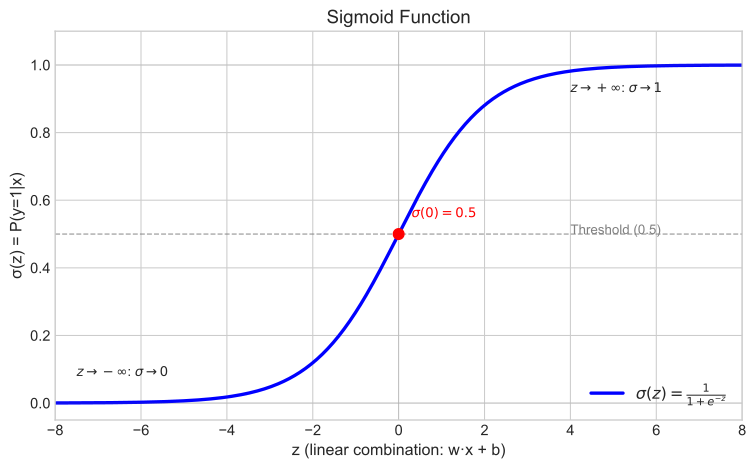
Why Sigmoid?

Property	Benefit
Maps $R \to (0, 1)$	Interpretable as probability
S-shaped curve	Captures threshold behavior
Nice derivative: $σ^{'} (z) = σ (z) (1 - σ (z))$	Efficient gradient computation

Decision Boundary

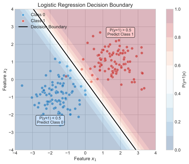
Predict $y = 1$ if $P (y = 1 | x) > 0.5$ , i.e., $w \cdot x + b > 0$
The decision boundary is the hyperplane $w \cdot x + b = 0$

Decision Boundary

Loss Function

Why Not MSE?

MSE loss with sigmoid creates a non-convex optimization problem with many local minima.

Cross-Entropy Loss (Log Loss)

L (w) = - \frac{1}{n} \sum_{i = 1}^{n} [y_{i} \log ({\hat{y}}_{i}) + (1 - y_{i}) \log (1 - {\hat{y}}_{i})]

where ${\hat{y}}_{i} = σ (w \cdot x_{i} + b)$

Cross-Entropy Loss

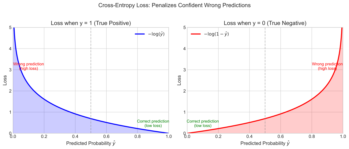
Intuition:

Scenario	Loss
$y = 1$ , $\hat{y} \to 1$	$\to 0$ (correct, confident)
$y = 1$ , $\hat{y} \to 0$	$\to \infty$ (wrong, confident)
$y = 0$ , $\hat{y} \to 0$	$\to 0$ (correct, confident)
$y = 0$ , $\hat{y} \to 1$	$\to \infty$ (wrong, confident)

Maximum Likelihood Interpretation

Cross-entropy equals negative log-likelihood under Bernoulli distribution:

P (y | x) = {\hat{y}}^{y} (1 - \hat{y})^{1 - y}

\log L = y \log (\hat{y}) + (1 - y) \log (1 - \hat{y})

Minimizing cross-entropy = Maximizing likelihood

Optimization

Gradient Descent

\frac{\partial L}{\partial w} = \frac{1}{n} \sum_{i = 1}^{n} ({\hat{y}}_{i} - y_{i}) x_{i}

Remarkably similar to linear regression gradient!

python

def logistic_regression_gd(X, y, lr=0.01, n_iters=1000):
    n, d = X.shape
    w = np.zeros(d)
    b = 0

    for _ in range(n_iters):
        z = X @ w + b
        y_pred = 1 / (1 + np.exp(-z))

        dw = (1/n) * X.T @ (y_pred - y)
        db = (1/n) * np.sum(y_pred - y)

        w -= lr * dw
        b -= lr * db

    return w, b

Newton's Method

For faster convergence, use second-order optimization:

w_{n e w} = w - H^{- 1} \nabla L

Pros: Converges in fewer iterations
Cons: Each iteration is $O (d^{3})$ due to Hessian inversion

Regularization

Type	Formula	Effect
L2 (Ridge)	$L + λ \| w \|_{2}^{2}$	Prevents large weights
L1 (Lasso)	$L + λ \| w \|_{1}$	Produces sparse weights (feature selection)

sklearn's C Parameter

sklearn uses $C = 1 / λ$ :

Large C: Less regularization, more complex model
Small C: More regularization, simpler model

Multiclass Extension

One-vs-Rest (OvR)

Train $k$ binary classifiers:

Classifier 1: Class 1 vs rest
Classifier 2: Class 2 vs rest
...

Prediction: Class with highest probability

Softmax Regression (Multinomial)

Generalizes sigmoid to $k$ classes:

P (y = j | x) = \frac{e^{w_{j} \cdot x}}{\sum_{k = 1}^{K} e^{w_{k} \cdot x}}

Loss: Categorical cross-entropy

L = - \sum_{i = 1}^{n} \sum_{j = 1}^{k} y_{i j} \log P (y = j | x_{i})

Key Properties

Assumptions

Assumption	Description
Linearity in log-odds	$\log \frac{p}{1 - p} = w \cdot x$ is linear
Independence	Observations are independent
No multicollinearity	Features not perfectly correlated
Large sample size	MLE needs sufficient data

Strengths vs Weaknesses

Strengths	Weaknesses
Probabilistic output (confidence scores)	Linear decision boundary only
Interpretable coefficients (odds ratios)	Requires feature engineering for non-linearity
Efficient: $O (n d)$ per iteration	Sensitive to outliers
Built-in regularization	Class imbalance issues
No distributional assumptions on $X$

Coefficient Interpretation

Log-Odds

\log \frac{p}{1 - p} = w_{0} + w_{1} x_{1} + w_{2} x_{2} + \dots

$w_{j}$ = change in log-odds for one-unit increase in $x_{j}$

Odds Ratio

Odds Ratio for x_{j} = e^{w_{j}}

Odds Ratio	Interpretation
$> 1$	Feature increases odds of positive class
$< 1$	Feature decreases odds
$= 1$	No effect

Example: If $w_{1} = 0.5$ for "years_experience":

Odds ratio $= e^{0.5} \approx 1.65$
"Each additional year increases odds of success by 65%"

Interview Questions

Q1: Why logistic over linear regression for classification?

Key points:

Bounded output - Linear regression can predict outside $[0, 1]$
Probabilistic interpretation - Calibrated probabilities for ranking/thresholding
Proper loss function - Cross-entropy correctly penalizes confident mistakes

Q2: How to handle class imbalance?

Approach	Description
Class weights	Upweight minority class (`class_weight='balanced'`)
Threshold adjustment	Don't use 0.5; tune based on precision-recall
Resampling	SMOTE, undersampling (after train/test split!)
Different metrics	Use precision, recall, F1, PR-AUC instead of accuracy

Q3: Non-linear relationships?

Options (in order of complexity):

Feature engineering (polynomial, interaction terms)
Generalized additive models (GAMs)
Non-linear models (trees, neural networks)

Q4: Sigmoid vs Softmax?

Sigmoid	Softmax
Single value $\to (0, 1)$	Vector of $k$ values $\to k$ probabilities summing to 1
Binary classification	Multiclass classification
$σ (z)$	$softmax ([z_{1}, \dots, z_{k}])_{j} = \frac{e^{z_{j}}}{\sum_{k} e^{z_{k}}}$

For binary: softmax $([z, 0])$ = $[σ (z), 1 - σ (z)]$

Code Reference

python

import numpy as np

class LogisticRegression:
    def __init__(self, lr=0.01, n_iters=1000, regularization='l2', lambda_=0.1):
        self.lr = lr
        self.n_iters = n_iters
        self.regularization = regularization
        self.lambda_ = lambda_
        self.weights = None
        self.bias = None

    def sigmoid(self, z):
        return 1 / (1 + np.exp(-np.clip(z, -500, 500)))

    def fit(self, X, y):
        n, d = X.shape
        self.weights = np.zeros(d)
        self.bias = 0

        for _ in range(self.n_iters):
            z = X @ self.weights + self.bias
            y_pred = self.sigmoid(z)

            # Gradients
            dw = (1/n) * X.T @ (y_pred - y)
            db = (1/n) * np.sum(y_pred - y)

            # Regularization
            if self.regularization == 'l2':
                dw += (self.lambda_ / n) * self.weights
            elif self.regularization == 'l1':
                dw += (self.lambda_ / n) * np.sign(self.weights)

            # Update
            self.weights -= self.lr * dw
            self.bias -= self.lr * db

    def predict_proba(self, X):
        return self.sigmoid(X @ self.weights + self.bias)

    def predict(self, X, threshold=0.5):
        return (self.predict_proba(X) >= threshold).astype(int)


class SoftmaxRegression:
    """Multiclass logistic regression."""
    def __init__(self, lr=0.01, n_iters=1000):
        self.lr = lr
        self.n_iters = n_iters
        self.weights = None

    def softmax(self, z):
        exp_z = np.exp(z - np.max(z, axis=1, keepdims=True))
        return exp_z / np.sum(exp_z, axis=1, keepdims=True)

    def fit(self, X, y):
        n, d = X.shape
        k = len(np.unique(y))
        y_onehot = np.zeros((n, k))
        y_onehot[np.arange(n), y] = 1
        self.weights = np.zeros((d, k))

        for _ in range(self.n_iters):
            y_pred = self.softmax(X @ self.weights)
            self.weights -= self.lr * (1/n) * X.T @ (y_pred - y_onehot)

    def predict(self, X):
        return np.argmax(self.softmax(X @ self.weights), axis=1)

Quick Reference Card

LOGISTIC REGRESSION
-----------------------------------------------------
Model:    P(y=1|x) = sigma(w.x + b)
Sigmoid:  sigma(z) = 1/(1 + e^(-z))
Loss:     Cross-entropy = -[y log(y_hat) + (1-y) log(1-y_hat)]
Gradient: dL/dw = (1/n) sum (y_hat - y)x

DECISION BOUNDARY
-----------------------------------------------------
Linear: w.x + b = 0
Predict y=1 if w.x + b > 0

MULTICLASS
-----------------------------------------------------
OvR:     Train k binary classifiers
Softmax: P(y=j|x) = e^(w_j.x) / sum_k e^(w_k.x)

INTERPRETATION
-----------------------------------------------------
w_j = change in log-odds per unit increase in x_j
e^(w_j) = odds ratio for x_j

USE WHEN
-----------------------------------------------------
- Binary/multiclass classification
- Need probability estimates
- Want interpretable coefficients
- Linear decision boundary is sufficient

Logistic Regression ​

One-Sentence Summary ​

Core Formulation ​

Model ​

Why Sigmoid? ​

Decision Boundary ​

Loss Function ​

Why Not MSE? ​

Cross-Entropy Loss (Log Loss) ​

Maximum Likelihood Interpretation ​

Optimization ​

Gradient Descent ​

Newton's Method ​

Regularization ​

sklearn's C Parameter ​

Multiclass Extension ​

One-vs-Rest (OvR) ​

Softmax Regression (Multinomial) ​

Key Properties ​

Assumptions ​

Strengths vs Weaknesses ​

Coefficient Interpretation ​

Log-Odds ​

Odds Ratio ​

Interview Questions ​

Q1: Why logistic over linear regression for classification? ​

Q2: How to handle class imbalance? ​

Q3: Non-linear relationships? ​

Q4: Sigmoid vs Softmax? ​

Code Reference ​

Quick Reference Card ​

Logistic Regression

One-Sentence Summary

Core Formulation

Model

Why Sigmoid?

Decision Boundary

Loss Function

Why Not MSE?

Cross-Entropy Loss (Log Loss)

Maximum Likelihood Interpretation

Optimization

Gradient Descent

Newton's Method

Regularization

sklearn's C Parameter

Multiclass Extension

One-vs-Rest (OvR)

Softmax Regression (Multinomial)

Key Properties

Assumptions

Strengths vs Weaknesses

Coefficient Interpretation

Log-Odds

Odds Ratio

Interview Questions

Q1: Why logistic over linear regression for classification?

Q2: How to handle class imbalance?

Q3: Non-linear relationships?

Q4: Sigmoid vs Softmax?

Code Reference

Quick Reference Card