Attention Fundamentals

Attention is a mechanism that allows neural networks to dynamically focus on relevant parts of an input sequence, overcoming the fixed-capacity bottleneck of recurrent architectures.

The Problem: RNN Bottleneck

Vanishing Gradients in Long Sequences

Recurrent Neural Networks (RNNs) process sequences sequentially, maintaining a hidden state that passes information from one timestep to the next. However, this sequential processing creates a critical problem: when backpropagating gradients through many timesteps, the gradients exponentially decay or explode.

Consider a sequence of length $T$. During backpropagation through time (BPTT), the gradient at timestep $t$ involves a chain of products:

$$\frac{\partial L}{\partial h_t}=\frac{\partial L}{\partial h_T}\cdot \frac{\partial h_T}{\partial h_{T-1}}\cdot \frac{\partial h_{T-1}}{\partial h_{T-2}}\cdots \frac{\partial h_{t+1}}{\partial h_t}$$

If each Jacobian matrix $\frac{\partial h_i}{\partial h_{i-1}}$ has spectral norm less than 1, the product of $(T-t)$ such matrices shrinks exponentially, making $\frac{\partial L}{\partial h_t}\approx 0$. This is the vanishing gradient problem. Conversely, if spectral norms exceed 1, gradients explode.

The practical consequence: RNNs struggle to learn long-range dependencies in text. Early tokens in a long sentence have minimal influence on later tokens because gradient signals decay exponentially over time steps.

Information Compression Problem

Beyond gradients, RNNs face an architectural limitation: all information from a sequence of length $T$ must be compressed into a fixed-size hidden state $h_T$ of dimension $d_{hidden}$. This creates an information bottleneck.

Consider translating a sentence with an RNN encoder-decoder model:

• The encoder processes the entire source sentence and outputs a single context vector $c=h_T$
• The decoder receives this single vector to generate all target words

For long sentences (20+ words), this single vector must preserve all semantic, syntactic, and lexical information. In practice, the model forgets early words or rare details that appear early in sequences.

This architectural constraint makes RNNs fundamentally inefficient for capturing complex dependencies across long ranges.

The Solution: Attention

The Key Insight

Rather than forcing all information through a fixed bottleneck, what if the decoder could look back at all encoder states, not just the final one? The attention mechanism enables exactly this.

The fundamental idea: Use the decoder's current state to compute a weighted average of all encoder states. The weights are learned dynamically—the model learns which input positions are relevant for generating the current output token.

For a decoder state $s_t$, instead of conditioning only on $h_T$, we compute:

$$c_t=\sum _{i=1}^T{\alpha }_{t,i}{h}_i$$

where ${\alpha }_{t,i}$ is the attention weight. The weights $\sum _i{\alpha }_{t,i}=1$ form a probability distribution over input positions, learned via a small neural network (the attention function).

This simple change has profound implications:

• No information bottleneck: Each decoder step attends directly to all encoder states
• Long-range dependencies: Direct connections bypass the sequential bottleneck
• Interpretability: Attention weights show which input words influenced each output word

Historical Context: Bahdanau vs. Luong

Two seminal approaches emerged in early attention research:

Bahdanau Attention (2015): Uses an additive scoring function (also called concat-based attention):

$${\alpha }_{t,i}=\frac{\exp (v^T\tanh (W_q{s}_t+W_k{h}_i))}{\sum _j\exp (v^T\tanh (W_q{s}_j+W_k{h}_j))}$$

This approach computes an intermediate representation by concatenating and transforming the query and key, then using a learned weight vector $v$ to score the result.

Luong Attention (2015): Uses a multiplicative (dot-product) scoring function:

$$\text{score}(s_t,h_i)=s_t^{T}W{h}_i$$

This is simpler and more computationally efficient. Luong attention later evolved into the scaled dot-product attention used in Transformers.

Both approaches produce nearly identical results in practice, but multiplicative attention became standard due to its computational efficiency and natural compatibility with matrix operations on GPUs.

Basic Attention Formula

The Attention Mechanism Deconstructed

The attention mechanism consists of three conceptual components, each serving a specific purpose:

1. Scoring Function (How relevant is this input position?)

Given a query $q$ (decoder state) and a key $k$ (encoder state), compute a compatibility score:

Scoring Method	Formula	Complexity
Dot-Product	$\text{score}(q,k)=q\cdot k$	$O(d)$
Scaled Dot-Product	$\text{score}(q,k)=\frac{q\cdot k}{\sqrt{d_k}}$	$O(d)$
Additive	$\text{score}(q,k)=v^T\tanh (W_{q}q+W_{k}k)$	$O(d^2)$
Bilinear	$\text{score}(q,k)=q^{T}Wk$	$O(d^2)$

The dot-product scoring is used in Transformers. The scaling factor $\frac{1}{\sqrt{d_k}}$ is crucial: when dimensionality $d_k$ is large, dot products grow large, pushing softmax into flat regions where gradients vanish. Scaling stabilizes training.

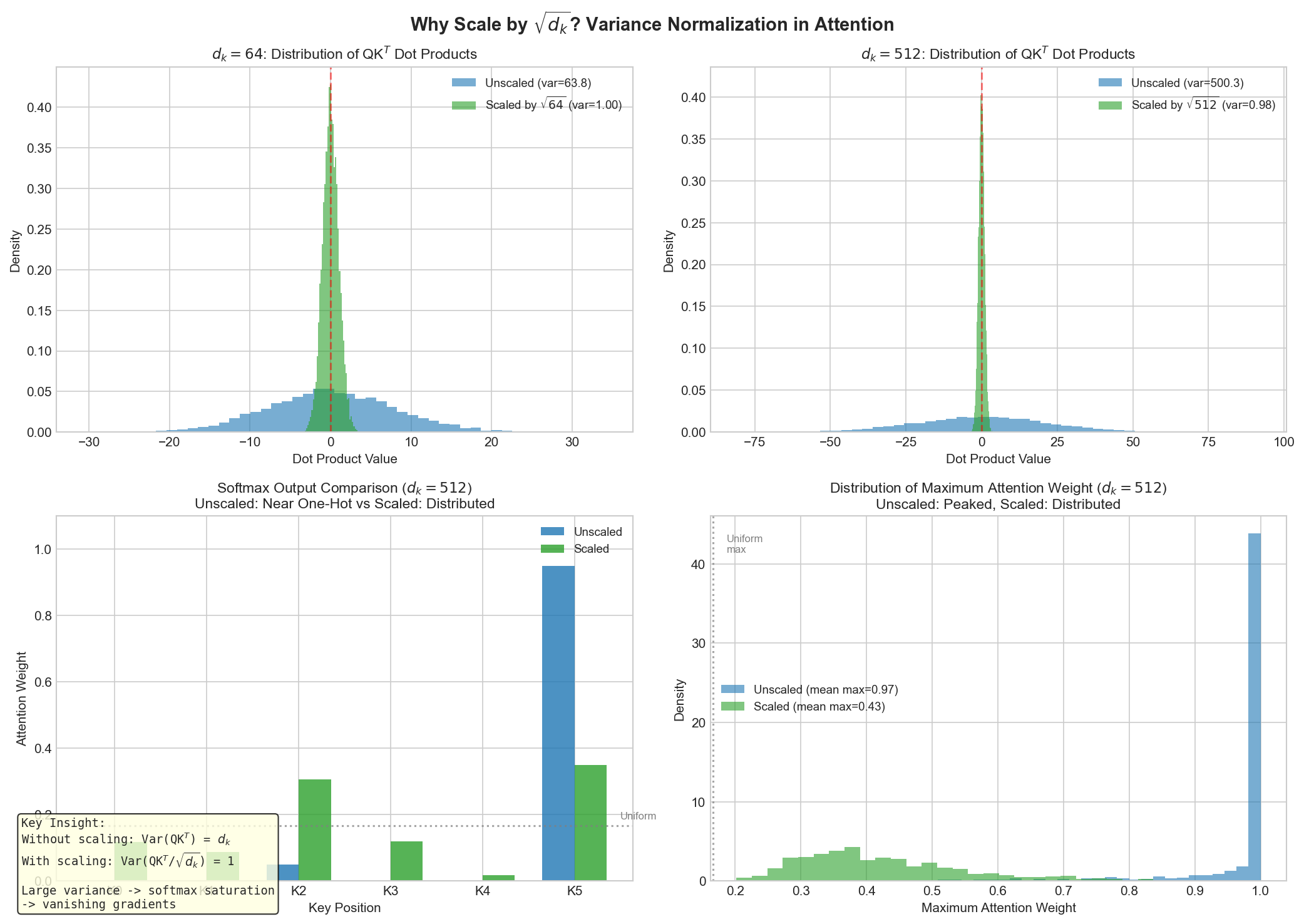
2. Softmax Normalization (Converting scores to probabilities)

Raw scores are often large or negative. We normalize them using softmax to create a probability distribution:

$${\alpha }_i={\text{softmax}}_i(\text{scores})=\frac{\exp ({\text{score}}_i)}{\sum _j\exp ({\text{score}}_j)}$$

The softmax function ensures:

• All weights are positive: ${\alpha }_i>0$
• Weights sum to 1: $\sum _i{\alpha }_i=1$
• Differentiable: Gradients flow during backpropagation
• Sharp focus: High-scoring positions receive exponentially more weight than low-scoring ones

Softmax is a "soft" version of argmax (hard selection), allowing the model to learn a smooth, differentiable attention mechanism.

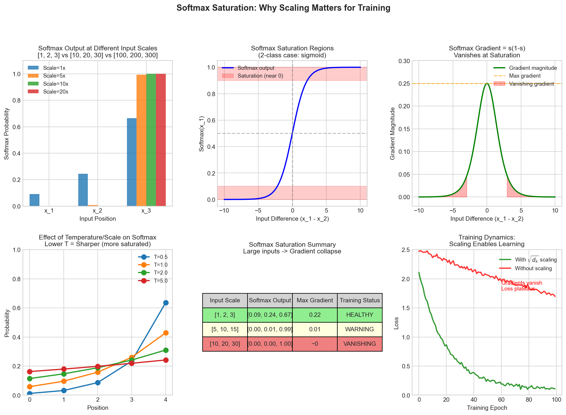
3. Context Vector Computation (Weighted aggregation)

The normalized weights multiply the values (another projection of encoder states):

$$c=\sum _i{\alpha }_i{v}_i$$

where $v_i$ is the value corresponding to the $i$-th position. In practice, $q$, $k$, and $v$ are learned linear projections of the encoder and decoder states.

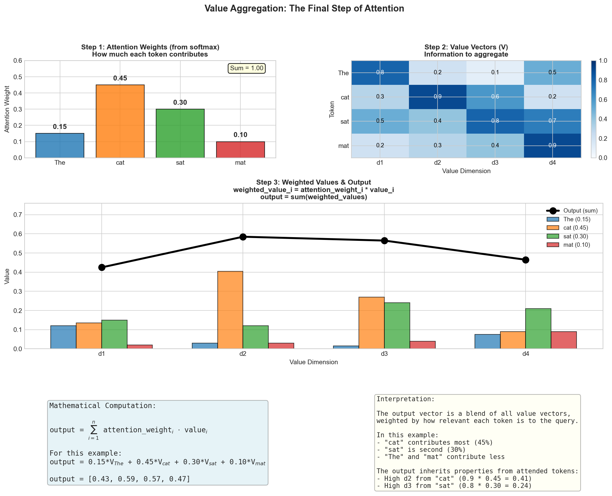
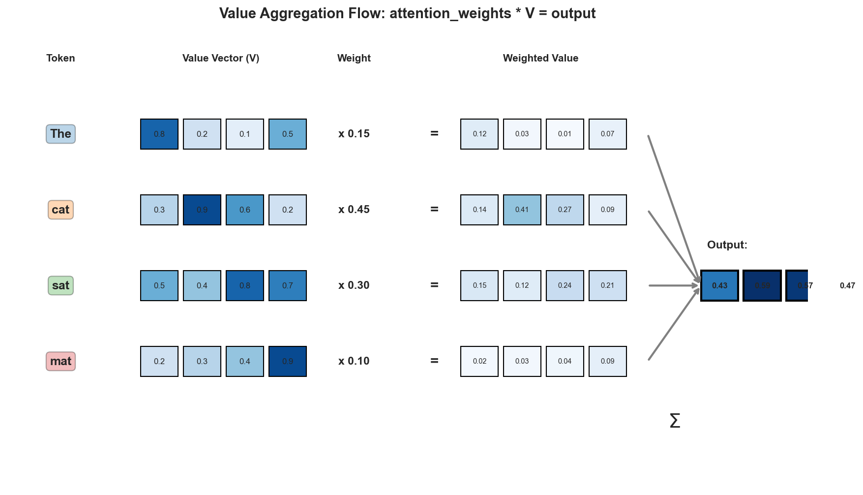
Complete Attention Computation

Combining these steps in matrix form:

$$\text{Attention}(Q,K,V)=\text{softmax}\left(\frac{Q{K}^T}{\sqrt{d_k}}\right)V$$

Here:

• $Q$ is a matrix of queries (decoder states), shape $[T_q,d_k]$
• $K$ is a matrix of keys (encoder states), shape $[T_k,d_k]$
• $V$ is a matrix of values (encoder states), shape $[T_k,d_v]$
• Output shape: $[T_q,d_v]$

This formula is the foundation for all attention mechanisms, including multi-head attention (Module 3) and self-attention in Transformers (Module 2).

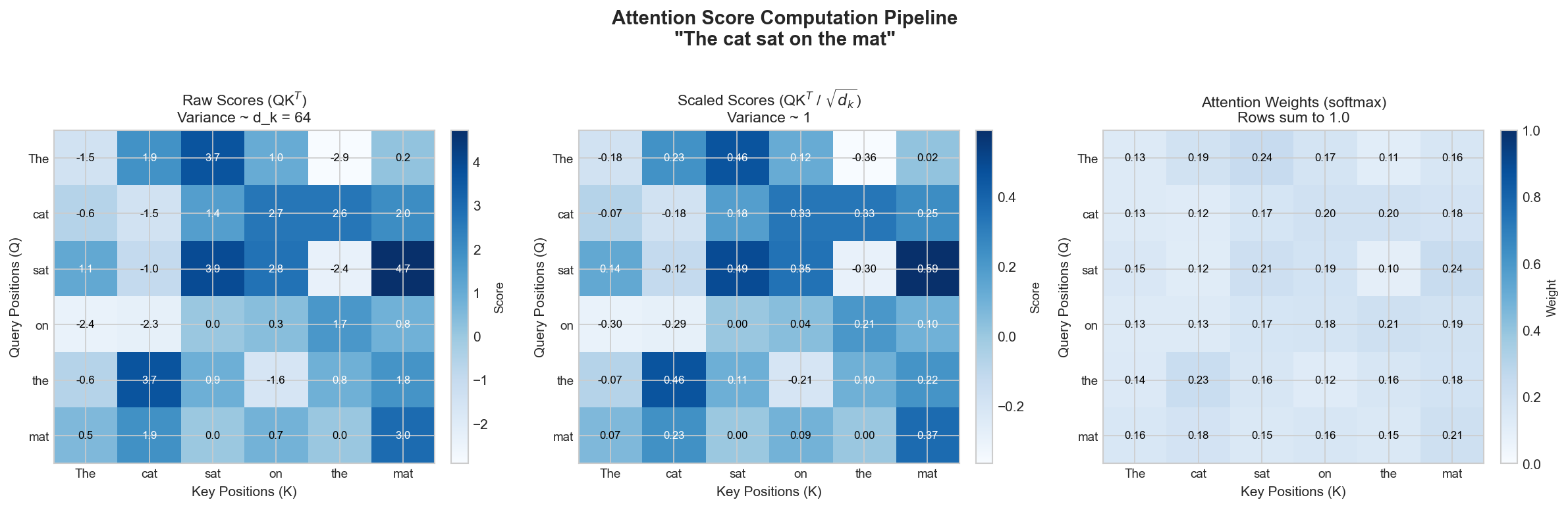
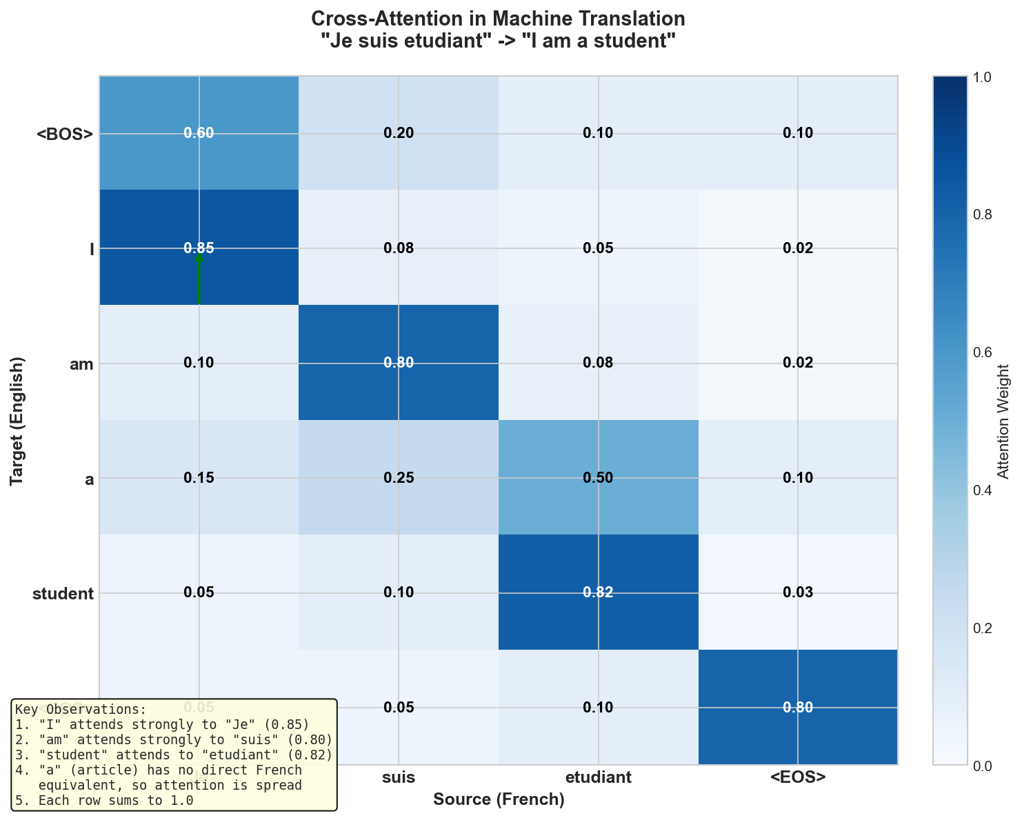
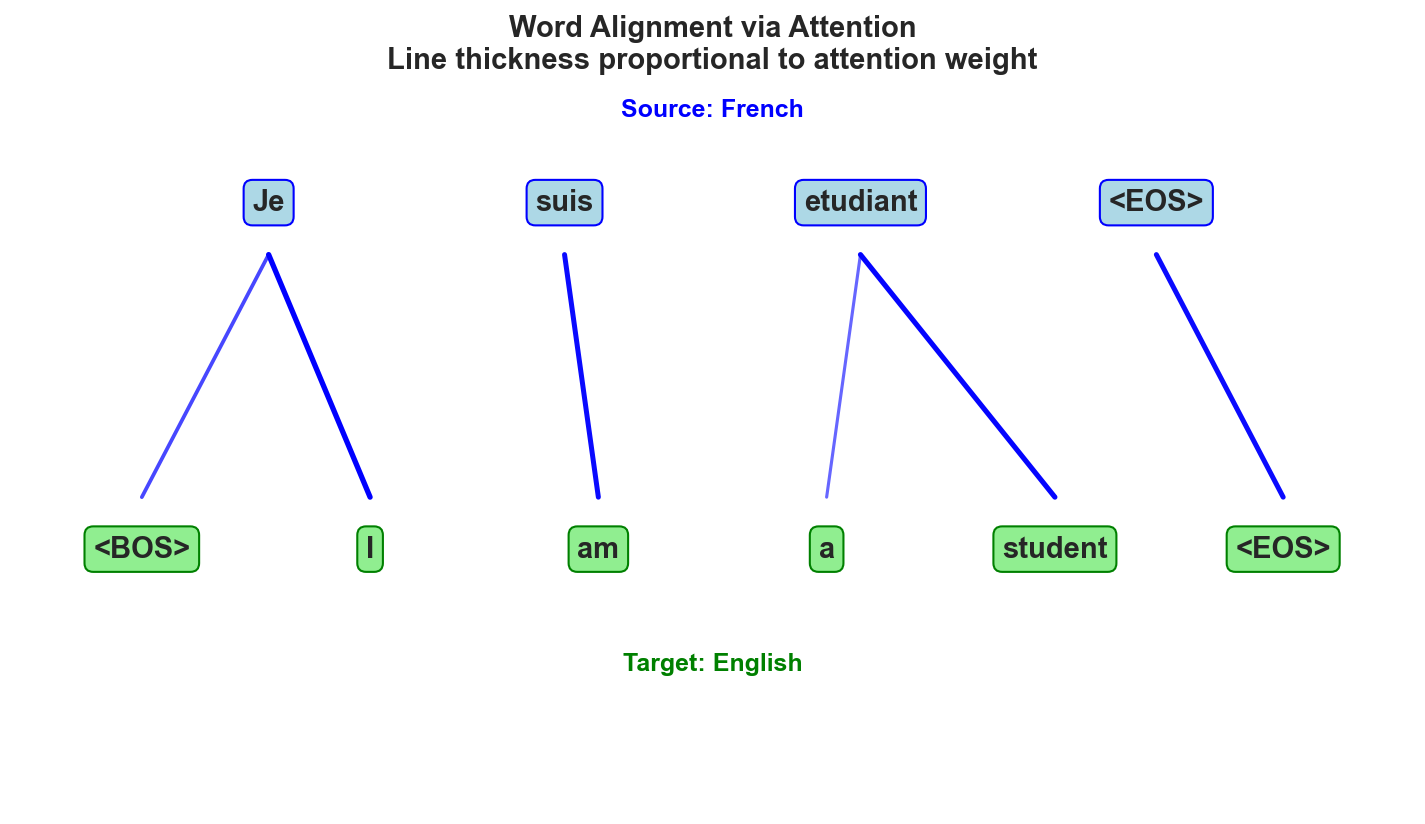
Practical Insight: Attention weight values are interpretable. In machine translation, an attention weight of 0.8 on the 3rd input word means the model is allocating 80% of focus to generating the current output word based on that input word. This interpretability is one reason Transformers became popular in industry.

Interview Questions

Question 1: Why does attention solve the vanishing gradient problem?

Sample Answer:

Attention creates direct connections from the decoder to all encoder positions, bypassing the sequential bottleneck of RNNs.

With vanilla RNNs, the gradient path from output word $t$ to input word 1 requires passing through $(t-1)$ timesteps, accumulating products of Jacobians:

$$\text{gradient path length}=O(T)$$

With attention, any decoder state can directly attend to any encoder state through a single attention computation. The gradient path becomes:

$$\frac{\partial L}{\partial h_i}\text{ has direct path of length }O(1)$$

Specifically, the loss gradient flows directly through the attention weights ${\alpha }_{i,j}$ without multiplicative decay. While attention still requires learning which positions matter, it doesn't suffer exponential decay.

However, we must be precise: attention doesn't eliminate gradient issues entirely. Softmax normalization and subsequent projections still require proper scaling (e.g., the $\sqrt{d_k}$ denominator). But the mechanism fundamentally reshapes the computation graph to avoid the exponential decay problem inherent to sequential processing.

Follow-up consideration: LSTM and GRU gates also address vanishing gradients through architectural gating. Attention complements these approaches by adding long-range connectivity.

Question 2: Explain the difference between additive (Bahdanau) and multiplicative (Luong/dot-product) attention. When would you use each?

Sample Answer:

Additive Attention (Bahdanau):

• Scoring function: $\text{score}(q,k)=v^T\tanh (W_{q}q+W_{k}k)$
• Computes a learned transformation of the concatenated query and key
• Requires two weight matrices ($W_q$, $W_k$) and a weight vector ($v$)
• More parameters and higher computational cost: $O(d^2)$
• Can capture more complex interactions between query and key

Multiplicative Attention (Luong/Dot-Product):

• Scoring function: $\text{score}(q,k)=q^{T}Wk$ (bilinear) or $q\cdot k$ (dot-product)
• Requires fewer parameters (one weight matrix or none)
• Computational cost: $O(d)$ for dot-product, $O(d^2)$ for bilinear
• More efficient, especially for large embedding dimensions
• Naturally parallelizable on modern hardware (GPUs, TPUs)

When to use each:

Use additive attention when:

• Computational resources are not constrained
• You have smaller embedding dimensions ($d<128$)
• You need maximum expressiveness for complex alignment patterns
• You're working in an academic setting where efficiency isn't critical

Use multiplicative attention when:

• You're building production systems with high throughput requirements
• Embedding dimensions are large ($d>256$)
• You want to leverage GPU/TPU acceleration
• You prioritize computational efficiency
• You're implementing Transformers (the standard choice)

Empirical note: Modern research shows dot-product attention with proper scaling ($\frac{1}{\sqrt{d_k}}$) is nearly identical to additive attention in practice, but it's orders of magnitude faster. This is why Transformers universally adopted scaled dot-product attention.

Question 3: How does attention handle variable-length sequences and padding? Why is masking important?

Sample Answer:

In practice, sequences in a batch have different lengths. For computational efficiency, we pad shorter sequences to match the longest sequence in the batch, introducing padding tokens.

The Problem with Naïve Attention:

Without masking, the attention mechanism will compute weights for padding tokens:

$${\alpha }_i=\frac{\exp ({\text{score}}_i)}{\sum _j\exp ({\text{score}}_j)}$$

Since softmax normalizes across all positions, including padding, the model can attend to padding tokens. This is problematic because:

1. Padding tokens contain no semantic information
2. The model wastes attention capacity on meaningless positions
3. Gradients flow to and from padding positions, wasting computation

The Solution: Masking

Before applying softmax, we set the scores of padding positions to $-\mathrm{\infty }$:

$${\text{score}}_{\text{pad}}=-\mathrm{\infty }$$

This ensures $\exp (-\mathrm{\infty })=0$, so ${\alpha }_{\text{pad}}=0$ after softmax. The padded positions contribute nothing to the context vector.

In implementation:

scores = Q @ K.T / sqrt(d_k)
scores[padding_mask] = -1e9  # Large negative number approximates -∞
attention_weights = softmax(scores)
context = attention_weights @ V

Other Masking Scenarios:

• Decoder self-attention in autoregressive models: Mask future positions to prevent cheating. A decoder should only attend to previously generated tokens.
• Causal masking: Upper triangular masking ensures position $t$ can only attend to positions $\le t$.

Practical Impact: Without proper masking, model predictions are undefined on sequences with different lengths, and the model incorrectly learns from padding. With masking, the model becomes robust to variable-length inputs and focuses only on meaningful tokens.

Quick Reference Card

╔════════════════════════════════════════════════════════════════════════════╗
║                       ATTENTION FUNDAMENTALS CHEAT SHEET                  ║
╚════════════════════════════════════════════════════════════════════════════╝

┌─ PROBLEM: RNN BOTTLENECK ────────────────────────────────────────────────┐
│                                                                            │
│  Vanishing Gradients:   Gradient ≈ ∏(Jacobians) → decays exponentially   │
│  Information Bottleneck: All info compressed into single vector h_T       │
│  Sequential Processing: Can't parallelize, O(T) depth                     │
│                                                                            │
└────────────────────────────────────────────────────────────────────────────┘

┌─ ATTENTION EQUATION ─────────────────────────────────────────────────────┐
│                                                                            │
│    Attention(Q, K, V) = softmax(QK^T / √d_k) V                           │
│                                                                            │
│  Q: Queries (what to look for)     [batch_size, seq_len, d_k]           │
│  K: Keys (what can be found)        [batch_size, seq_len, d_k]           │
│  V: Values (information to take)    [batch_size, seq_len, d_v]           │
│  d_k: Key dimension                                                       │
│                                                                            │
│  Output: Context vectors             [batch_size, seq_len, d_v]          │
│                                                                            │
└────────────────────────────────────────────────────────────────────────────┘

┌─ SCORING FUNCTIONS ──────────────────────────────────────────────────────┐
│                                                                            │
│  Name              Formula                        Complexity  Best For   │
│  ─────────────────────────────────────────────────────────────────────   │
│  Dot-Product       q · k                          O(d)       Large d     │
│  Scaled DP         q · k / √d_k                   O(d)       Transformers│
│  Additive          v^T tanh(W_q q + W_k k)        O(d²)      Small d     │
│  Bilinear          q^T W k                        O(d²)      Flexibility │
│                                                                            │
└────────────────────────────────────────────────────────────────────────────┘

┌─ SOFTMAX NORMALIZATION ──────────────────────────────────────────────────┐
│                                                                            │
│  Purpose:  Convert scores to probability distribution [0, 1]             │
│  Formula:  α_i = exp(score_i) / Σ_j exp(score_j)                         │
│  Property: Σ_i α_i = 1                                                   │
│  Effect:   High scores → exponentially higher weights                    │
│           Focuses on top few positions                                    │
│                                                                            │
└────────────────────────────────────────────────────────────────────────────┘

┌─ CONTEXT VECTOR ─────────────────────────────────────────────────────────┐
│                                                                            │
│  Weighted aggregation of values:   c = Σ_i α_i v_i                      │
│                                                                            │
│  Intuition: Each output position gets a blend of input information,       │
│           weighted by how relevant each input is.                         │
│                                                                            │
│  Parallelizable: All positions computed simultaneously (O(1) depth)       │
│                                                                            │
└────────────────────────────────────────────────────────────────────────────┘

┌─ KEY IMPROVEMENTS OVER RNNs ─────────────────────────────────────────────┐
│                                                                            │
│  ✓ Direct connections bypass sequential bottleneck                        │
│  ✓ Path length: O(1) instead of O(T)                                      │
│  ✓ Fully parallelizable across sequence                                   │
│  ✓ Interpretable: attention weights show importance                       │
│  ✓ No information compression: attend to all positions                    │
│  ✓ Gradient flow: direct paths prevent vanishing gradients                │
│                                                                            │
└────────────────────────────────────────────────────────────────────────────┘

┌─ MASKING STRATEGIES ─────────────────────────────────────────────────────┐
│                                                                            │
│  Padding Mask:      Set scores of <pad> tokens to -∞                     │
│                    Prevents attending to padding                          │
│                                                                            │
│  Causal Mask:       Upper triangular: position t sees only t ≤ pos       │
│                    Required for autoregressive models                     │
│                                                                            │
│  Implementation:    scores[mask] = -1e9  (before softmax)                │
│                    Ensures α_masked ≈ 0 after softmax                    │
│                                                                            │
└────────────────────────────────────────────────────────────────────────────┘

┌─ HISTORICAL CONTEXT ─────────────────────────────────────────────────────┐
│                                                                            │
│  2014-2015: Bahdanau et al., Luong et al.                                │
│            RNN + Attention for machine translation                        │
│                                                                            │
│  2017: Vaswani et al.                                                    │
│       "Attention Is All You Need"                                        │
│       Scaled dot-product attention                                        │
│       Multi-head attention                                               │
│       Transformer architecture                                           │
│                                                                            │
└────────────────────────────────────────────────────────────────────────────┘

┌─ CONNECTING TO OTHER MODULES ────────────────────────────────────────────┐
│                                                                            │
│  Module 1 (Current): Single attention head, foundational concepts         │
│  Module 2:          Self-attention: Q, K, V all from same source          │
│  Module 3:          Multi-head attention: Parallel attention mechanisms   │
│  Module 4:          Positional encoding: Inject sequence position info    │
│  Module 5:          Full Transformer: Combine all components              │
│                                                                            │
└────────────────────────────────────────────────────────────────────────────┘

Visual Cheat Sheet

Key Takeaways

1. Attention solves the RNN bottleneck by providing direct connections between distant positions, enabling parallel computation and preventing vanishing gradients.

2. The attention formula (Attention(Q, K, V)) is elegantly simple: compute compatibility scores between queries and keys, normalize with softmax, and aggregate values using resulting weights.

3. Scaled dot-product attention is the standard due to computational efficiency while maintaining expressiveness equivalent to more complex scoring functions.

4. Masking is critical for handling variable-length sequences and preventing the model from attending to meaningless padding or future tokens.

5. Attention is interpretable: The attention weights directly indicate which input positions influenced each output position, providing transparency many other neural components lack.

This module builds the foundation for self-attention (Module 2) and multi-head attention (Module 3), which are core to the Transformer architecture that has revolutionized NLP and beyond.