Policy Gradients

Learning policies directly — REINFORCE, the policy gradient theorem, and variance reduction

---

One-Sentence Summary

Policy gradients optimize a parameterized policy directly by estimating gradients of expected return through sampled trajectories, avoiding the need for explicit value function maximization.

---

Why Direct Policy Optimization?

Limitations of Value-Based Methods

Value-based methods (Q-learning, DQN) learn an action-value function $Q(s,a)$ and derive a policy implicitly:

$$\pi (s)=\arg \underset{a}{max}Q(s,a)$$

This approach has fundamental limitations:

Issue	Description
Discrete actions only	Argmax requires enumeration over all actions
Deterministic policies	Cannot represent stochastic behavior
High-dimensional actions	Intractable for continuous control
Indirect optimization	Optimizing $Q$ does not directly optimize policy performance

Advantages of Policy Gradients

Policy gradient methods parameterize the policy directly as ${\pi }_{\theta }(a|s)$ and optimize parameters $\theta$ to maximize expected return:

• Continuous actions: Natural representation via Gaussian policies
• Stochastic policies: Enable exploration and handle partial observability
• Direct optimization: Gradient ascent on the true objective
• Smoother optimization: Small $\theta$ changes yield small policy changes

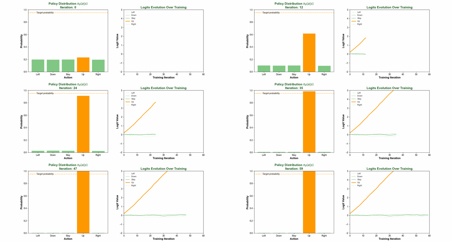
The animation shows how a policy evolves during training, with action probabilities shifting toward the optimal action as the agent learns.

---

Policy Parameterization

The Policy Network

A parameterized policy ${\pi }_{\theta }(a|s)$ maps states to action distributions:

Discrete Actions: Softmax Policy

For discrete action spaces, output logits and apply softmax:

$${\pi }_{\theta }(a|s)=\frac{\exp (f_{\theta }(s,a))}{\sum _{a^{\prime }}\exp (f_{\theta }(s,a^{\prime }))}$$

where $f_{\theta }(s,a)$ is the network output (logit) for action $a$.

Continuous Actions: Gaussian Policy

For continuous actions, output mean and variance of a Gaussian:

$${\pi }_{\theta }(a|s)=\mathcal{N}({\mu }_{\theta }(s),{\sigma }_{\theta }(s{)}^2)$$

The network outputs ${\mu }_{\theta }(s)$ (mean) and optionally $\log {\sigma }_{\theta }(s)$ (log standard deviation).

Log probability for gradients:

$$\log {\pi }_{\theta }(a|s)=-\frac{(a-{\mu }_{\theta }(s){)}^2}{2{\sigma }_{\theta }(s{)}^2}-\log {\sigma }_{\theta }(s)-\frac{1}{2}\log (2\pi )$$

---

The Policy Gradient Theorem

Objective Function

We want to maximize expected cumulative reward (return):

$$J(\theta )={\mathbb{E}}_{\tau \sim {\pi }_{\theta }}\left[\sum _{t=0}^T{\gamma }^t{r}_t\right]={\mathbb{E}}_{\tau \sim {\pi }_{\theta }}[R(\tau )]$$

where $\tau =(s_0,a_0,r_0,s_1,a_1,r_1,\dots )$ is a trajectory.

The Gradient

The key insight: we can compute the gradient of $J(\theta )$ even though the expectation is over trajectories that depend on $\theta$:

$${\mathrm{\nabla }}_{\theta }J(\theta )={\mathbb{E}}_{\tau \sim {\pi }_{\theta }}[R(\tau )\sum _{t=0}^T{\mathrm{\nabla }}_{\theta }\log {\pi }_{\theta }(a_t|s_t)]$$

Derivation Intuition

The derivation uses the log-derivative trick:

$${\mathrm{\nabla }}_{\theta }{\pi }_{\theta }(a|s)={\pi }_{\theta }(a|s){\mathrm{\nabla }}_{\theta }\log {\pi }_{\theta }(a|s)$$

Starting from the objective:

$$J(\theta )=\sum _{\tau }P(\tau |\theta )R(\tau )$$

Taking the gradient:

$${\mathrm{\nabla }}_{\theta }J(\theta )=\sum _{\tau }{\mathrm{\nabla }}_{\theta }P(\tau |\theta )R(\tau )$$

Applying the log-derivative trick:

$$=\sum _{\tau }P(\tau |\theta ){\mathrm{\nabla }}_{\theta }\log P(\tau |\theta )R(\tau )$$

Since $P(\tau |\theta )=p(s_0)\prod _t{\pi }_{\theta }(a_t|s_t)p(s_{t+1}|s_t,a_t)$, only the policy terms depend on $\theta$:

$${\mathrm{\nabla }}_{\theta }\log P(\tau |\theta )=\sum _{t=0}^T{\mathrm{\nabla }}_{\theta }\log {\pi }_{\theta }(a_t|s_t)$$

This yields the policy gradient theorem:

$$\boxed{{\displaystyle {\mathrm{\nabla }}_{\theta }J(\theta )={\mathbb{E}}_{\tau \sim {\pi }_{\theta }}[R(\tau )\sum _{t=0}^T{\mathrm{\nabla }}_{\theta }\log {\pi }_{\theta }(a_t|s_t)]}}$$

Key insight: The gradient is an expectation, so we can estimate it by sampling trajectories.

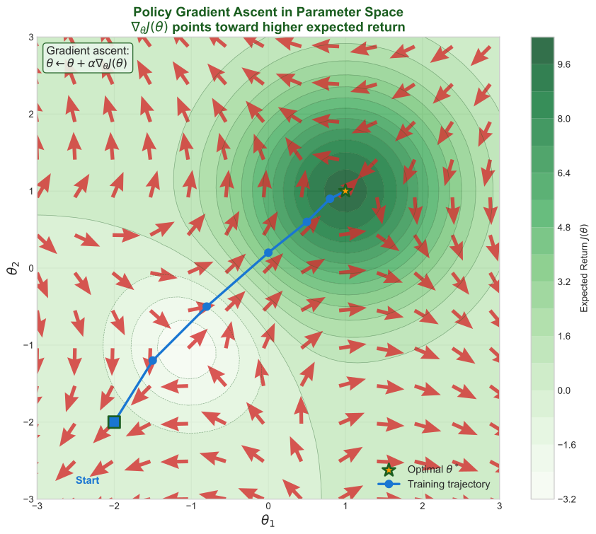
Policy gradient ascent in parameter space: arrows show gradient directions pointing toward regions of higher expected return.

---

REINFORCE Algorithm

Algorithm Overview

REINFORCE (Williams, 1992) is the simplest policy gradient algorithm:

Algorithm: REINFORCE
─────────────────────────────────────
1. Initialize policy parameters θ
2. For each episode:
   a. Generate trajectory τ = (s₀, a₀, r₀, ..., s_T)
   b. Compute return R(τ) = Σᵢ γⁱrᵢ
   c. For each timestep t:
      - Compute gradient: ĝ = R(τ) ∇_θ log π_θ(aₜ|sₜ)
      - Update: θ ← θ + α ĝ

Monte Carlo Estimation

The gradient estimate uses complete episodes (Monte Carlo):

$$\hat{g}=\frac{1}{N}\sum _{n=1}^{N}R({\tau }_n)\sum _{t=0}^T{\mathrm{\nabla }}_{\theta }\log {\pi }_{\theta }(a_t^n|s_t^n)$$

Properties:

• Unbiased: $\mathbb{E}[\hat{g}]={\mathrm{\nabla }}_{\theta }J(\theta )$
• High variance: Single trajectory estimates are noisy
• On-policy: Requires fresh samples after each update

Causality Improvement

Actions at time $t$ cannot affect rewards at earlier times. We can use reward-to-go:

$${\mathrm{\nabla }}_{\theta }J(\theta )=\mathbb{E}[\sum _{t=0}^T{\mathrm{\nabla }}_{\theta }\log {\pi }_{\theta }(a_t|s_t)\sum _{t^{\prime }=t}^T{\gamma }^{t^{\prime }-t}{r}_{t^{\prime }}]$$

This uses $G_t=\sum _{t^{\prime }=t}^T{\gamma }^{t^{\prime }-t}{r}_{t^{\prime }}$ instead of $R(\tau )$, reducing variance.

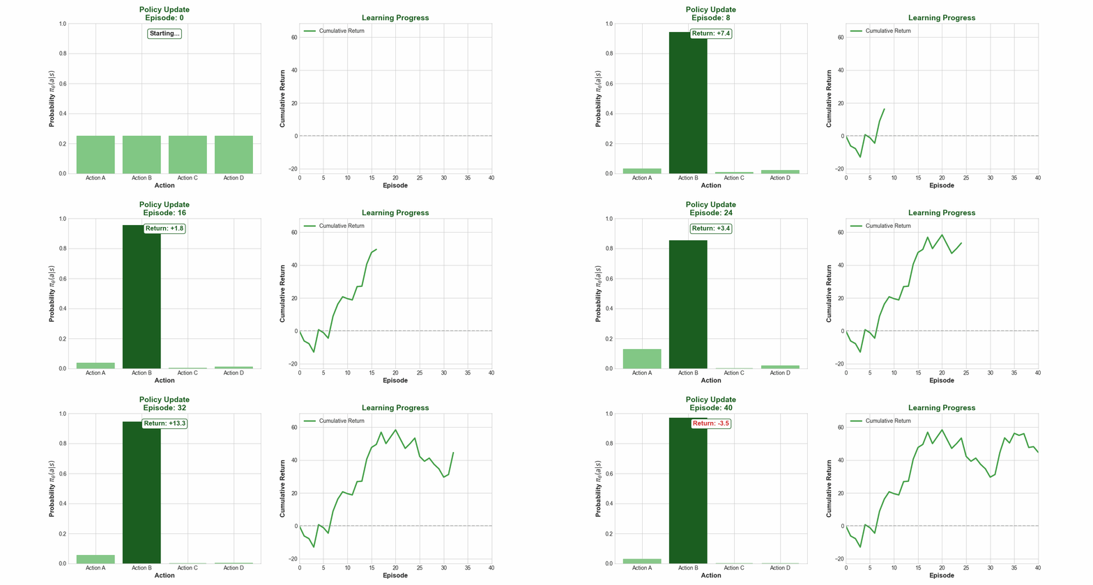
REINFORCE in action: the policy updates based on episode returns, gradually concentrating probability on better actions.

---

The Variance Problem

Why High Variance?

Policy gradient estimates suffer from high variance because:

1. Stochastic actions: Randomness in action sampling
2. Stochastic transitions: Environment dynamics
3. Rare events: Important but infrequent rewards

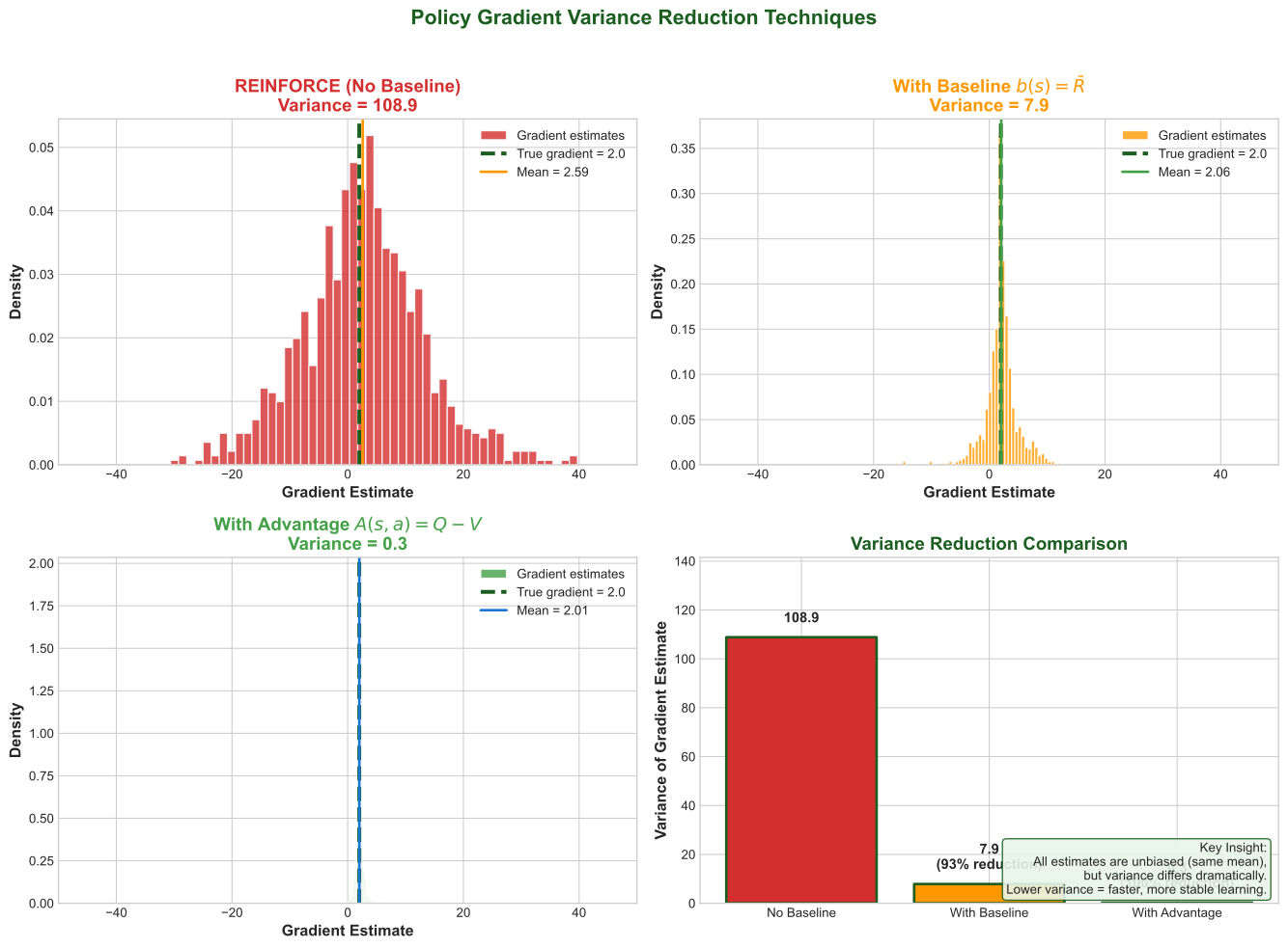
Consequence: Gradient estimates swing wildly between updates, causing unstable learning.

Baseline Subtraction

We can subtract any function $b(s)$ that does not depend on actions:

$${\mathrm{\nabla }}_{\theta }J(\theta )=\mathbb{E}[\sum _{t=0}^T{\mathrm{\nabla }}_{\theta }\log {\pi }_{\theta }(a_t|s_t)(G_t-b(s_t))]$$

Why this works: The subtracted term has zero expectation:

$${\mathbb{E}}_{a\sim {\pi }_{\theta }}[{\mathrm{\nabla }}_{\theta }\log {\pi }_{\theta }(a|s)\cdot b(s)]=b(s)\sum _a{\mathrm{\nabla }}_{\theta }{\pi }_{\theta }(a|s)=b(s){\mathrm{\nabla }}_{\theta }\underset{=1}{\underbrace{\sum _a{\pi }_{\theta }(a|s)}}=0$$

Common Baselines

Baseline	Formula	Variance Reduction
Constant	$b=\overline{R}$ (average return)	Moderate
State-dependent	$b(s)=V(s)$ (value function)	High
Moving average	$b=\text{EMA}(R)$	Moderate

Optimal baseline: The value function $V^{\pi }(s)$ is provably the variance-minimizing baseline.

---

The Advantage Function

Definition

The advantage function measures how much better an action is compared to the average:

$$A^{\pi }(s,a)=Q^{\pi }(s,a)-V^{\pi }(s)$$

where:

• $Q^{\pi }(s,a)$ = expected return starting from $(s,a)$ following $\pi$
• $V^{\pi }(s)$ = expected return starting from $s$ following $\pi$

Advantage Actor-Critic Gradient

Using advantage as the weighting term:

$${\mathrm{\nabla }}_{\theta }J(\theta )=\mathbb{E}[\sum _{t=0}^T{\mathrm{\nabla }}_{\theta }\log {\pi }_{\theta }(a_t|s_t)A^{\pi }(s_t,a_t)]$$

Intuition:

• $A>0$: Action better than average — increase probability
• $A<0$: Action worse than average — decrease probability
• $A=0$: Action is average — no change

Advantage Estimation

Since we do not know the true advantage, we estimate it:

TD(0) Advantage Estimate:

$${\hat{A}}_t=r_t+\gamma V(s_{t+1})-V(s_t)$$

Generalized Advantage Estimation (GAE):

$${\hat{A}}_t^{\text{GAE}(\gamma ,\lambda )}=\sum _{l=0}^{\mathrm{\infty }}(\gamma \lambda {)}^l{\delta }_{t+l}$$

where ${\delta }_t=r_t+\gamma V(s_{t+1})-V(s_t)$ is the TD error.

GAE interpolates between high-bias/low-variance ($\lambda =0$) and low-bias/high-variance ($\lambda =1$).

---

Policy Gradients for Continuous Actions

Gaussian Policy Implementation

For continuous control, we typically use a diagonal Gaussian:

$${\pi }_{\theta }(a|s)=\mathcal{N}({\mu }_{\theta }(s),\text{diag}({\sigma }_{\theta }^2))$$

The network outputs:

• Mean: ${\mu }_{\theta }(s)$ — deterministic component
• Log std: $\log \sigma$ — learned or fixed

Score Function for Gaussian

The gradient of log probability:

$${\mathrm{\nabla }}_{\theta }\log {\pi }_{\theta }(a|s)={\mathrm{\nabla }}_{\theta }{\mu }_{\theta }(s)\cdot \frac{a-{\mu }_{\theta }(s)}{{\sigma }^2}+{\mathrm{\nabla }}_{\theta }\log {\sigma }_{\theta }(s)\cdot (\frac{(a-{\mu }_{\theta }(s){)}^2}{{\sigma }^2}-1)$$

Interpretation:

• If $a>\mu$: Increase $\mu$ to make $a$ more likely
• Magnitude scales inversely with ${\sigma }^2$ (more certain = larger gradients)

Exploration-Exploitation

Approach	Method	Trade-off
Entropy bonus	Add $H[{\pi }_{\theta }(·|s)]$ to objective	Encourages exploration
Fixed variance	$\sigma$ is a hyperparameter	Simpler but less adaptive
Learned variance	Network outputs $\log \sigma$	Adapts exploration over time

---

Visual Summary

---

Interview Questions

Q1: "Why do we need the log-derivative trick in policy gradients?"

Answer:

The log-derivative trick converts a gradient of a probability distribution into an expectation we can sample from.

The problem: We want ${\mathrm{\nabla }}_{\theta }{\mathbb{E}}_{a\sim {\pi }_{\theta }}[R]$, but the expectation itself depends on $\theta$:

$${\mathrm{\nabla }}_{\theta }\sum _a{\pi }_{\theta }(a)R(a)$$

The solution: Using ${\mathrm{\nabla }}_{\theta }\pi =\pi {\mathrm{\nabla }}_{\theta }\log \pi$:

$$=\sum _a{\pi }_{\theta }(a){\mathrm{\nabla }}_{\theta }\log {\pi }_{\theta }(a)R(a)={\mathbb{E}}_{a\sim {\pi }_{\theta }}[R(a){\mathrm{\nabla }}_{\theta }\log {\pi }_{\theta }(a)]$$

Now we can estimate this gradient by sampling actions from our policy. Without this trick, we would need to compute gradients through the sampling process itself, which is not differentiable.

---

Q2: "What is the advantage function and why does it reduce variance?"

Answer:

The advantage function $A^{\pi }(s,a)=Q^{\pi }(s,a)-V^{\pi }(s)$ measures how much better action $a$ is compared to the average action under policy $\pi$ in state $s$.

Variance reduction mechanism:

1. Centering: By subtracting $V(s)$, we center the reward signal around zero. Good actions get positive weights, bad actions get negative weights.

2. Credit assignment: Instead of weighting by absolute return (which includes rewards unrelated to the current action), we weight by relative performance.

3. Reduced scale: Returns can be very large or vary wildly across episodes. Advantage values are typically smaller and more consistent.

Example: If baseline return is 100 and we get 102, raw weighting uses 102 while advantage uses +2. The smaller magnitude means less variance in gradient estimates.

---

Q3: "Compare REINFORCE to Actor-Critic. When would you use each?"

Answer:

Aspect	REINFORCE	Actor-Critic
Value function	None	Learned critic $V(s)$
Bias	Unbiased	Biased (critic error)
Variance	High (Monte Carlo)	Lower (TD estimates)
Sample efficiency	Low	Higher
Complexity	Simple	Two networks to train

Use REINFORCE when:

• Episodes are short (low variance naturally)
• Simplicity is prioritized
• Debugging/understanding the algorithm

Use Actor-Critic when:

• Episodes are long (need variance reduction)
• Sample efficiency matters
• Continuous control tasks
• Building toward PPO/A3C

Key insight: Actor-Critic trades unbiasedness for variance reduction. The bias introduced by an imperfect critic is usually preferable to the high variance of REINFORCE in practice.

---

Quick Reference Card

POLICY GRADIENT CORE
─────────────────────────────────────────────────────────────
Objective:     J(θ) = E_τ[R(τ)]
Gradient:      ∇J = E[R(τ) Σ_t ∇log π_θ(aₜ|sₜ)]
Log-trick:     ∇π = π ∇log π

REINFORCE
─────────────────────────────────────────────────────────────
Update:        θ ← θ + α R(τ) ∇log π_θ(a|s)
Reward-to-go:  Use Gₜ = Σ_{t'≥t} γ^(t'-t) r_{t'}
Properties:    Unbiased, high variance, on-policy

VARIANCE REDUCTION
─────────────────────────────────────────────────────────────
Baseline:      Subtract b(s) — zero expected gradient
Best baseline: V^π(s) — value function
Advantage:     A(s,a) = Q(s,a) - V(s)

CONTINUOUS ACTIONS
─────────────────────────────────────────────────────────────
Gaussian:      π(a|s) = N(μ_θ(s), σ²)
Log-prob:      -½[(a-μ)²/σ²] - log σ - ½log(2π)
Exploration:   Entropy bonus, learned σ

ALGORITHMS HIERARCHY
─────────────────────────────────────────────────────────────
REINFORCE → Actor-Critic → A2C/A3C → PPO/TRPO
(simple)     (baseline)     (parallel)  (constrained)

---

Key Takeaways

1. Policy gradients optimize policies directly by computing gradients of expected return through sampled trajectories, enabling continuous actions and stochastic policies.

2. The policy gradient theorem provides an unbiased gradient estimate using the log-derivative trick: weight each action's score function by its return.

3. Variance is the central challenge — REINFORCE estimates are unbiased but noisy. Baselines and advantage functions dramatically reduce variance without introducing bias.

4. The advantage function measures relative action quality, providing both variance reduction and intuitive credit assignment.

5. Actor-Critic methods trade a small amount of bias (from critic errors) for significant variance reduction, forming the foundation for modern algorithms like PPO and A3C.