Regularization

Fighting overfitting — techniques to improve generalization

Why Regularization?

Neural networks have millions of parameters — enough to memorize training data perfectly. Regularization prevents overfitting by adding constraints that encourage simpler models.

The Overfitting Problem

Overfitting Curves

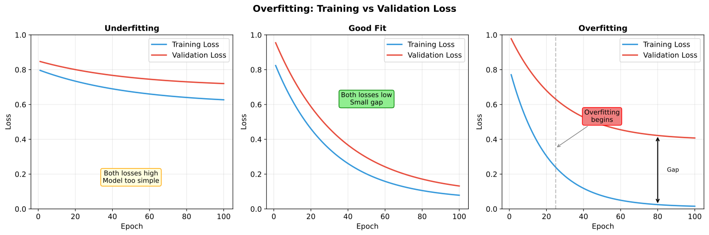
Sign	Indication
Training loss ↓, Validation loss ↑	Overfitting
Training loss high	Underfitting
Both losses low and close	Good fit

Bias-Variance Perspective

Regularization trades bias (underfitting) for reduced variance (overfitting). The goal is to find the sweet spot.

L2 Regularization (Weight Decay)

Add squared magnitude of weights to the loss:

L_{t o t a l} = L_{d a t a} + λ \sum_{i} w_{i}^{2}

Effect on Optimization

Gradient becomes: $\nabla L = \nabla L_{d a t a} + 2 λ w$

Update: $w = w - α (\nabla L_{d a t a} + 2 λ w) = (1 - 2 α λ) w - α \nabla L_{d a t a}$

The $(1 - 2 α λ)$ factor shrinks weights toward zero each step — hence "weight decay."

Why It Works

Smaller weights → smoother function → less overfitting
Bayesian view: L2 regularization is equivalent to a Gaussian prior on weights
Prevents any single weight from dominating

Typical Values

$λ = 1 e - 4$ to $1 e - 2$
Start with $1 e - 4$ , increase if overfitting persists

L1 Regularization

Add absolute magnitude of weights:

L_{t o t a l} = L_{d a t a} + λ \sum_{i} | w_{i} |

L1 vs L2

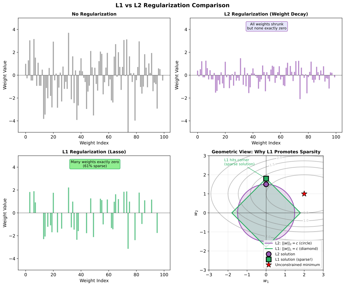
Aspect	L1	L2
Effect	Pushes weights to exactly zero	Shrinks all weights
Sparsity	Yes (feature selection)	No
Prior	Laplace	Gaussian
Gradient	Constant magnitude	Proportional to weight

When to Use L1

When you want sparse solutions (many zero weights)
Feature selection: L1 automatically selects important features
Often combined with L2 (Elastic Net): $λ_{1} | | w | |_{1} + λ_{2} | | w | |_{2}^{2}$

Dropout

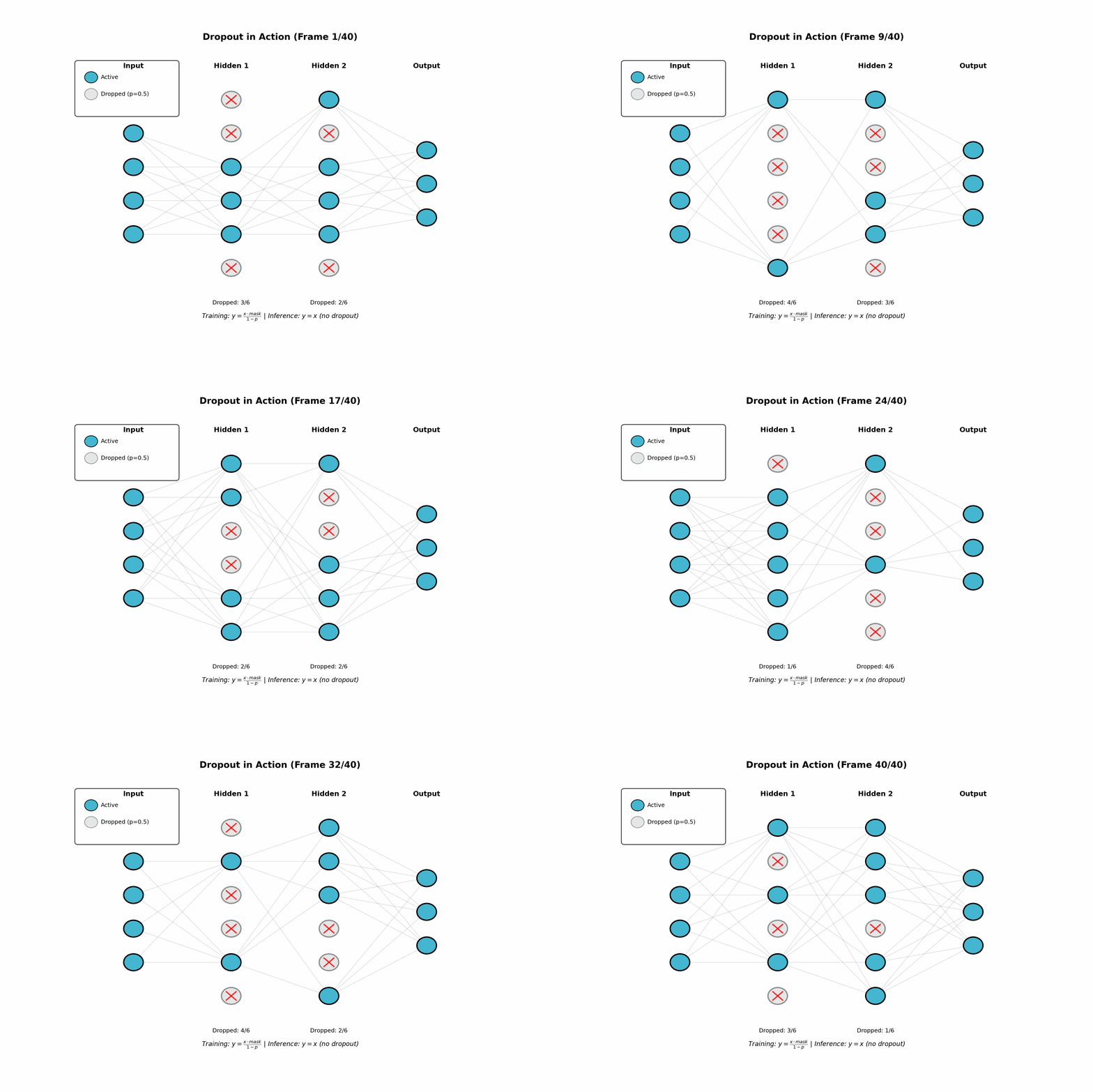
Randomly zero out neurons during training.

Algorithm

python

def dropout(x, p=0.5, training=True):
    if not training:
        return x
    mask = (torch.rand_like(x) > p).float()
    return x * mask / (1 - p)  # Scale to maintain expected value

Training vs Inference

Phase	Behavior
Training	Randomly drop neurons with probability $p$
Inference	Use all neurons (no dropout)

The scaling by $1 / (1 - p)$ during training ensures expected output is unchanged at inference (called inverted dropout).

Dropout Animation

Why Dropout Works

Prevents co-adaptation: Neurons can't rely on specific other neurons
Ensemble effect: Each dropout mask creates a different subnetwork
Implicit regularization: Similar to training an ensemble of models

Typical Dropout Rates

Layer Type	Dropout Rate
After fully connected	0.5
After conv layers	0.1-0.25
In transformers (attention)	0.1
Input layer	0.2 (if used)

Early Stopping

Stop training when validation loss stops improving.

Algorithm

python

best_val_loss = float('inf')
patience_counter = 0
patience = 10  # Number of epochs to wait

for epoch in range(max_epochs):
    train_loss = train_one_epoch()
    val_loss = validate()

    if val_loss < best_val_loss:
        best_val_loss = val_loss
        save_checkpoint()
        patience_counter = 0
    else:
        patience_counter += 1

    if patience_counter >= patience:
        break  # Early stop

# Load best checkpoint for final model
load_checkpoint()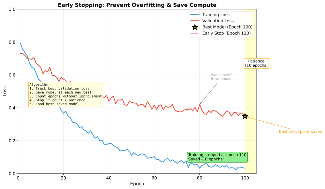

Early Stopping

Considerations

Patience: How many epochs to wait (typically 5-20)
What to monitor: Usually validation loss, sometimes validation metric
Save best model: Always save checkpoint at best validation performance

Data Augmentation

Artificially increase training data by applying transformations.

Image Augmentation

Transform	Effect
Random crop	Translation invariance
Horizontal flip	Mirror invariance
Color jitter	Lighting robustness
Rotation	Rotation invariance
Cutout/RandomErasing	Occlusion robustness

Advanced Techniques

Mixup: Interpolate between training examples

\tilde{x} = λ x_{i} + (1 - λ) x_{j}

\tilde{y} = λ y_{i} + (1 - λ) y_{j}

CutMix: Cut and paste patches between images

AutoAugment: Learned augmentation policies

Text Augmentation

Back-translation: Translate to another language and back
Synonym replacement: Replace words with synonyms
Random insertion/deletion: Add or remove words

Other Techniques

Label Smoothing

Instead of hard targets [0, 0, 1, 0], use soft targets [0.025, 0.025, 0.925, 0.025]:

y_{s m o o t h} = (1 - ϵ) \cdot y_{o n e h o t} + \frac{ϵ}{K}

Why it helps: Prevents model from being overconfident, improves calibration.

Batch Normalization as Regularization

BatchNorm adds noise through batch statistics, acting as implicit regularization:

Each sample's normalization depends on other samples in batch
Different batches produce different normalizations

Stochastic Depth

Randomly skip entire layers during training (like dropout for layers):

Used in deep residual networks
Reduces training time
Regularization effect

Combining Regularizers

Typical Combinations

Model Type	Regularization Stack
CNN	BatchNorm + Dropout (0.5 on FC) + Weight Decay + Data Augmentation
Transformer	LayerNorm + Dropout (0.1) + Weight Decay
MLP	Dropout (0.5) + Weight Decay

Diminishing Returns

Adding more regularization has diminishing returns. If model still overfits:

Get more data (best solution)
Reduce model capacity
Use stronger augmentation

Tuning Strategy

Start with standard defaults (BatchNorm, small weight decay)
Monitor train/val gap
If overfitting: add dropout, increase weight decay
If underfitting: reduce regularization, increase capacity

Interview Questions

Q1: "Explain the difference between L1 and L2 regularization."

L2 regularization ( $λ \sum w^{2}$ ):
Gradient: $2 λ w$ (proportional to weight)
Effect: Shrinks all weights toward zero, but rarely exactly zero
Result: Many small weights
Prior: Gaussian (prefers weights near zero)
L1 regularization ( $λ \sum | w |$ ):
Gradient: $λ \cdot sign (w)$ (constant magnitude)
Effect: Pushes weights exactly to zero
Result: Sparse weights (many exactly zero)
Prior: Laplace (sharp peak at zero)
When to use:
L2: Default choice, when all features are relevant
L1: Feature selection, when you want sparse models
Elastic Net (L1 + L2): When you want some sparsity with stability

Q2: "How does dropout prevent overfitting?"

Three perspectives:
Prevents co-adaptation: Neurons can't rely on specific other neurons being present. Each neuron must learn robust features independently.
Ensemble effect: Each dropout mask creates a different subnetwork. Training with dropout is like training an ensemble of $2^{n}$ networks (where n = number of neurons). At inference, using all neurons approximates averaging the ensemble.
Noise injection: Dropout adds noise to hidden representations, similar to data augmentation but in feature space. This prevents the model from fitting noise in the training data.
Implementation detail: Scale activations by $1 / (1 - p)$ during training so that expected values match inference (inverted dropout).
Typical rates: 0.5 for fully connected, 0.1-0.25 for conv layers.

Q3: "How do you choose regularization strength?"

Use validation performance as the guide:
Start with defaults:
Weight decay: 1e-4
Dropout: 0.5 (FC), 0.1 (attention)
Monitor train/val gap:
Large gap → increase regularization
Both losses high → decrease regularization
Grid search or random search:
Weight decay: [1e-5, 1e-4, 1e-3, 1e-2]
Dropout: [0.1, 0.3, 0.5]
Early stopping is almost always good:
Low cost, significant benefit
Use patience of 5-20 epochs
Data augmentation before other regularization:
More effective than weight penalties
No cost at inference time
Red flag: If you need very strong regularization, consider whether the model is too large for your data.

Key Takeaways

L2 (weight decay) shrinks weights — default regularization for most cases.
L1 creates sparse solutions — use for feature selection.
Dropout prevents co-adaptation — essential for fully connected layers.
Early stopping is free regularization — always use validation-based stopping.
Data augmentation is powerful — often more effective than weight penalties.
Combine techniques but watch for diminishing returns — more data beats more regularization.

Regularization ​

Why Regularization? ​

The Overfitting Problem ​

Bias-Variance Perspective ​

L2 Regularization (Weight Decay) ​

Effect on Optimization ​

Why It Works ​

Typical Values ​

L1 Regularization ​

L1 vs L2 ​

When to Use L1 ​

Dropout ​

Algorithm ​

Training vs Inference ​

Why Dropout Works ​

Typical Dropout Rates ​

Early Stopping ​

Algorithm ​

Considerations ​

Data Augmentation ​

Image Augmentation ​

Advanced Techniques ​

Text Augmentation ​

Other Techniques ​

Label Smoothing ​

Batch Normalization as Regularization ​

Stochastic Depth ​

Combining Regularizers ​

Typical Combinations ​

Diminishing Returns ​

Tuning Strategy ​

Interview Questions ​

Q1: "Explain the difference between L1 and L2 regularization." ​

Q2: "How does dropout prevent overfitting?" ​

Q3: "How do you choose regularization strength?" ​

Key Takeaways ​

Regularization

Why Regularization?

The Overfitting Problem

Bias-Variance Perspective

L2 Regularization (Weight Decay)

Effect on Optimization

Why It Works

Typical Values

L1 Regularization

L1 vs L2

When to Use L1

Dropout

Algorithm

Training vs Inference

Why Dropout Works

Typical Dropout Rates

Early Stopping

Algorithm

Considerations

Data Augmentation

Image Augmentation

Advanced Techniques

Text Augmentation

Other Techniques

Label Smoothing

Batch Normalization as Regularization

Stochastic Depth

Combining Regularizers

Typical Combinations

Diminishing Returns

Tuning Strategy

Interview Questions

Q1: "Explain the difference between L1 and L2 regularization."

Q2: "How does dropout prevent overfitting?"

Q3: "How do you choose regularization strength?"

Key Takeaways