Support Vector Machines (SVM)

Maximum margin classifiers - margins, kernels, soft margin

---

One-Sentence Description

SVM finds the hyperplane that maximizes the margin between classes, with kernel tricks enabling non-linear decision boundaries.

---

Core Concept: Maximum Margin

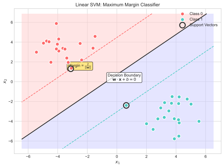
What is Margin?

The margin is the distance between the decision boundary and the nearest data points from either class (support vectors).

Why Maximize Margin?

Benefit	Explanation
Better generalization	More room for error on new data
Unique solution	Maximum margin hyperplane is unique
Robustness	Less sensitive to small perturbations

Support Vectors

• Data points closest to the decision boundary
• They "support" (define) the boundary
• Key insight: Only support vectors matter - other points can be removed without changing the solution

---

Mathematical Formulation

Hard Margin SVM (Linearly Separable Data)

Objective: Find $\mathbf{w}$, $b$ that maximize margin $=\frac{2}{\parallel \mathbf{w}\parallel }$

Optimization Problem:

$$\underset{\mathbf{w},b}{min}\frac{1}{2}\parallel \mathbf{w}{\parallel }^2$$$$\text{subject to: }{y}_i(\mathbf{w}\cdot {\mathbf{x}}_i+b)\ge 1\mathrm{\forall }i$$

This is a convex quadratic programming problem with a unique solution.

Soft Margin SVM (Non-Separable Data)

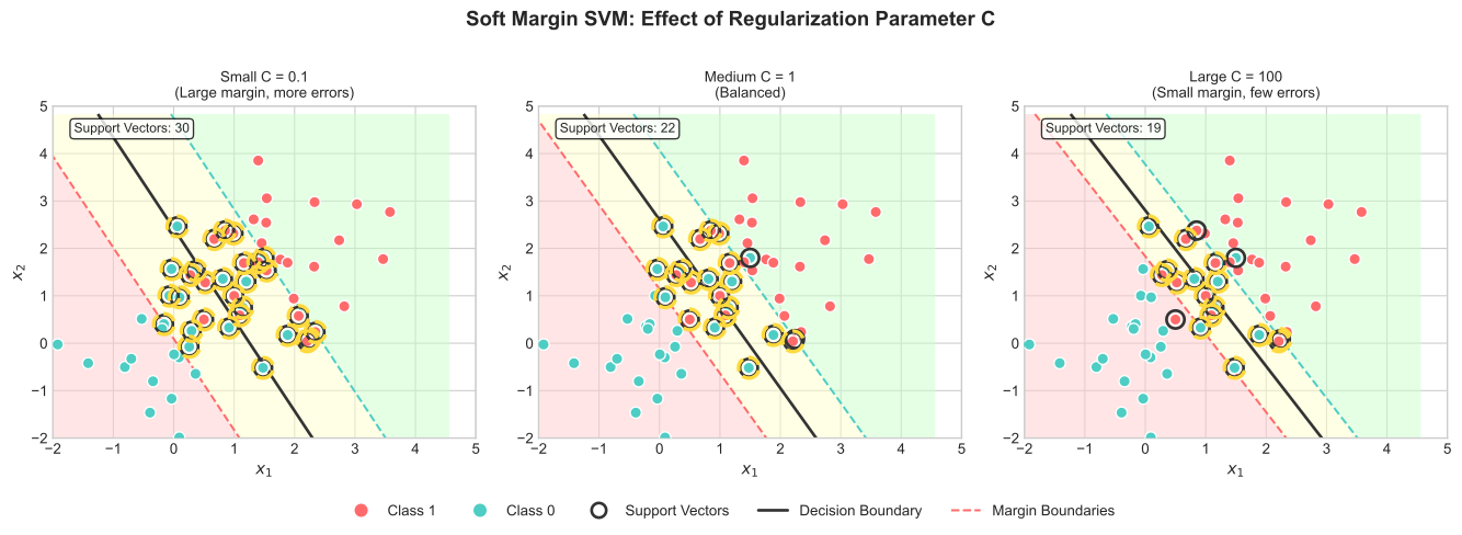
Allow some misclassification via slack variables ${\xi }_i$:

$$\underset{\mathbf{w},b,\xi }{min}\frac{1}{2}\parallel \mathbf{w}{\parallel }^2+C\sum _i{\xi }_i$$$$\text{subject to: }{y}_i(\mathbf{w}\cdot {\mathbf{x}}_i+b)\ge 1-{\xi }_i,{\xi }_i\ge 0$$

C Parameter Effect:

C Value	Margin	Errors	Risk
Large C	Smaller	Fewer	Overfitting
Small C	Larger	More	Underfitting

---

Kernel Trick

The Problem

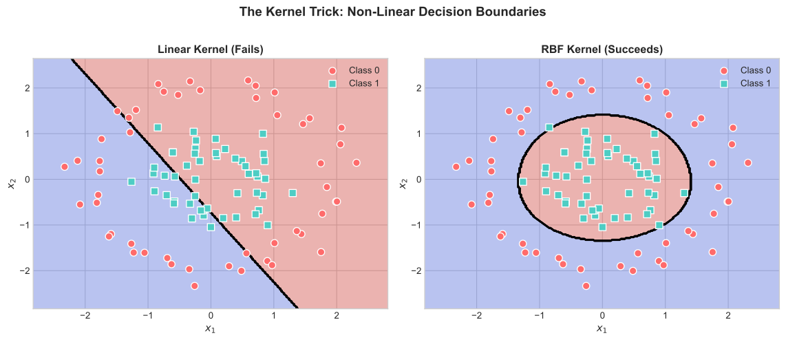
Linear SVM can only find linear decision boundaries. For non-linearly separable data, we need something more powerful.

The Solution

1. Map data to higher-dimensional space: $\varphi (\mathbf{x})$
2. Data may become linearly separable in higher dimensions
3. Use kernel trick to avoid computing $\varphi (\mathbf{x})$ explicitly

Kernel Function

$$K({\mathbf{x}}_i,{\mathbf{x}}_j)=\varphi ({\mathbf{x}}_i)\cdot \varphi ({\mathbf{x}}_j)$$

Computes dot product in high-dimensional space without explicitly transforming data.

Common Kernels

Kernel	Formula	Use Case
Linear	$K(\mathbf{x},\mathbf{y})=\mathbf{x}\cdot \mathbf{y}$	Linearly separable data
Polynomial	$K(\mathbf{x},\mathbf{y})=(\gamma \mathbf{x}\cdot \mathbf{y}+r{)}^d$	Polynomial boundaries
RBF/Gaussian	$K(\mathbf{x},\mathbf{y})=\exp (-\gamma |\mathbf{x}-\mathbf{y}{|}^2)$	Non-linear (most common)
Sigmoid	$K(\mathbf{x},\mathbf{y})=\tanh (\gamma \mathbf{x}\cdot \mathbf{y}+r)$	Neural network-like

RBF Kernel Parameter $\gamma$

$\gamma$ Value	Influence	Boundary	Risk
Large	Narrow	Complex	Overfitting
Small	Wide	Smooth	Underfitting

---

Hyperparameter Tuning

Key Parameters

Parameter	Description	Tuning Range
C	Regularization strength	$[0.01,0.1,1,10,100]$
kernel	Decision boundary type	'rbf', 'linear', 'poly'
$\gamma$	RBF kernel width	'scale', 'auto', $[0.01,0.1,1]$
degree	Polynomial kernel degree	$[2,3,4,5]$

Tuning Strategy

from sklearn.model_selection import GridSearchCV
from sklearn.svm import SVC

param_grid = {
    'C': [0.1, 1, 10, 100],
    'gamma': ['scale', 'auto', 0.1, 1, 10],
    'kernel': ['rbf', 'poly']
}

grid_search = GridSearchCV(SVC(), param_grid, cv=5, scoring='accuracy')
grid_search.fit(X_train, y_train)
print(f"Best params: {grid_search.best_params_}")

Common Pitfalls

• Always scale features - SVM uses distances, sensitive to scale
• Start with RBF kernel - Works well in most cases
• Use cross-validation for C and $\gamma$ - Default values rarely optimal

---

Key Properties

Strengths	Weaknesses
Effective in high dimensions ($d>n$)	Slow for large $n$: $O(n^2)$ to $O(n^3)$
Memory efficient (only stores SVs)	Requires feature scaling
Versatile (different kernels)	No native probability output
Robust to outliers (soft margin)	Kernel selection is difficult
Strong theoretical guarantees	Hard to interpret with kernels

---

Complexity Analysis

Operation	Time Complexity	Space Complexity
Training	$O(n^2)$ to $O(n^3)$	$O(n^2)$
Prediction	$O(n_{sv}\times d)$	$O(n_{sv}\times d)$

For large datasets, consider:

• Linear SVM (LinearSVC) - $O(n\times d)$
• SGD classifier with hinge loss
• Approximations (Nystrom, random features)

---

SVM vs Other Classifiers

Aspect	SVM	Logistic Regression
Objective	Maximize margin	Maximize likelihood
Probabilities	Not native	Natural
Kernels	Easy to apply	Requires explicit features
Scaling	Critical	Less sensitive
Large datasets	Slower	Faster

When to Use SVM

• High-dimensional data (text, genomics)
• $n_{features}>n_{samples}$
• Non-linear boundaries needed
• Medium-sized datasets (< 100K samples)

When to Avoid SVM

• Large datasets (use linear SVM or SGD)
• Need probability estimates (use logistic regression)
• Interpretability required (use linear models or trees)

---

Interview Questions

Q1: "Explain what the kernel trick does."

The kernel trick lets us compute dot products in a high-dimensional feature space without explicitly transforming data there.

SVM only needs dot products between data points, never the transformed features themselves. A kernel function $K({\mathbf{x}}_i,{\mathbf{x}}_j)=\varphi ({\mathbf{x}}_i)\cdot \varphi ({\mathbf{x}}_j)$ computes this directly, even when $\varphi$ maps to infinite dimensions (like RBF).

Example: The RBF kernel $K(\mathbf{x},\mathbf{y})=\exp (-\gamma \parallel \mathbf{x}-\mathbf{y}{\parallel }^2)$ implicitly maps to infinite dimensions but computes in $O(d)$ time.

Q2: "What's the role of C in SVM?"

C controls the trade-off between:

1. Maximizing the margin
2. Minimizing classification errors

• Large C: Prioritizes correct classification, smaller margin, risk of overfitting
• Small C: Prioritizes large margin, tolerates errors, better generalization

Tune C using cross-validation, typically searching powers of 10: $[0.01,0.1,1,10,100]$

Q3: "What are support vectors and why do they matter?"

Support vectors are training points on or within the margin boundary.

Why they matter:

1. Define the model - Decision boundary depends only on SVs
2. Sparse solution - Only store SVs for prediction
3. Complexity indicator - Many SVs suggests complex boundary or noisy data

Example: 10,000 training points but only 500 SVs means prediction uses only those 500 points.

Q4: "How would you handle a large dataset with SVM?"

Standard SVM is $O(n^2)$ to $O(n^3)$. For large datasets:

1. Linear SVM - LinearSVC is $O(n\times d)$ using coordinate descent
2. SGD with hinge loss - SGDClassifier(loss='hinge') scales to millions
3. Kernel approximations - Random Fourier features or Nystrom approximation
4. Subsampling - Train on a subset (loses information)

Start with linear SVM or SGD, then try kernel approximations if non-linear boundaries are necessary.

---

Code Reference

import numpy as np
from sklearn.svm import SVC
from sklearn.preprocessing import StandardScaler
from sklearn.model_selection import GridSearchCV

# Always scale features for SVM
scaler = StandardScaler()
X_train_scaled = scaler.fit_transform(X_train)
X_test_scaled = scaler.transform(X_test)

# Basic SVM
svm = SVC(kernel='rbf', C=1.0, gamma='scale')
svm.fit(X_train_scaled, y_train)

# With probability estimates
svm_prob = SVC(kernel='rbf', probability=True)
svm_prob.fit(X_train_scaled, y_train)
probs = svm_prob.predict_proba(X_test_scaled)

# Hyperparameter tuning
param_grid = {'C': [0.1, 1, 10, 100], 'gamma': [0.01, 0.1, 1, 'scale']}
grid_search = GridSearchCV(SVC(kernel='rbf'), param_grid, cv=5)
grid_search.fit(X_train_scaled, y_train)

# Access support vectors
print(f"Number of support vectors: {len(svm.support_vectors_)}")
print(f"Support vector indices: {svm.support_}")

---

Quick Reference Card

SVM Essentials
Goal	Maximize margin between classes
Decision Boundary	$\mathbf{w}\cdot \mathbf{x}+b=0$
Margin	$\frac{2}{|\mathbf{w}|}$

Soft Margin
Objective	$min\frac{1}{2}|\mathbf{w}{|}^2+C\sum _i{\xi }_i$
Large C	Fit training data, small margin
Small C	Large margin, allow errors

Kernels
Linear	$K(\mathbf{x},\mathbf{y})=\mathbf{x}\cdot \mathbf{y}$
Polynomial	$K(\mathbf{x},\mathbf{y})=(\gamma \mathbf{x}\cdot \mathbf{y}+r{)}^d$
RBF	$K(\mathbf{x},\mathbf{y})=\exp (-\gamma |\mathbf{x}-\mathbf{y}{|}^2)$

Complexity
Training	$O(n^2)$ to $O(n^3)$
Prediction	$O(n_{sv}\times d)$

Use When	Avoid When
High-dimensional data ($d>n$)	Large datasets
Non-linear boundaries needed	Need probability estimates
Medium-sized datasets	Interpretability required