RNNs, LSTM, and GRU

Processing sequences — from vanilla RNNs to gated architectures

---

The Sequential Data Problem

Many problems involve sequences: text, speech, time series, video. Standard neural networks fail because:

1. Variable length: Sentences have different numbers of words
2. Order matters: "dog bites man" ≠ "man bites dog"
3. Long-range dependencies: "The cat, which sat on the mat, was..."

Why MLPs Fail

• Fixed input size (can't handle variable length)
• No parameter sharing across positions
• No notion of temporal order

---

Vanilla RNN

RNNs maintain a hidden state that gets updated at each timestep, creating a "memory" of previous inputs.

Architecture

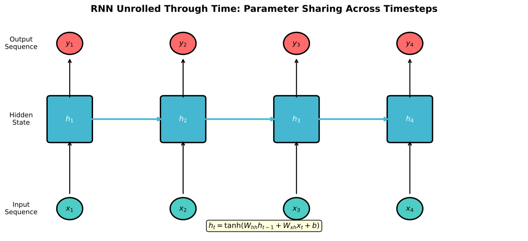
At each timestep $t$:

$$h_t=\tanh (W_{hh}{h}_{t-1}+W_{xh}{x}_t+b_h)$$$$y_t=W_{hy}{h}_t+b_y$$

Where:

• $x_t$ = input at time $t$
• $h_t$ = hidden state at time $t$
• $y_t$ = output at time $t$
• $W_{hh},W_{xh},W_{hy}$ = weight matrices (shared across time)

Parameter Sharing

The same weights are used at every timestep — this is what enables handling variable-length sequences.

Backpropagation Through Time (BPTT)

Unroll the RNN and apply standard backpropagation:

x₁ → x₂ → x₃ → ... → xₜ
↓     ↓     ↓           ↓
h₁ → h₂ → h₃ → ... → hₜ
↓     ↓     ↓           ↓
y₁    y₂    y₃         yₜ

Gradient flows backward through all timesteps.

---

The Vanishing Gradient Problem in RNNs

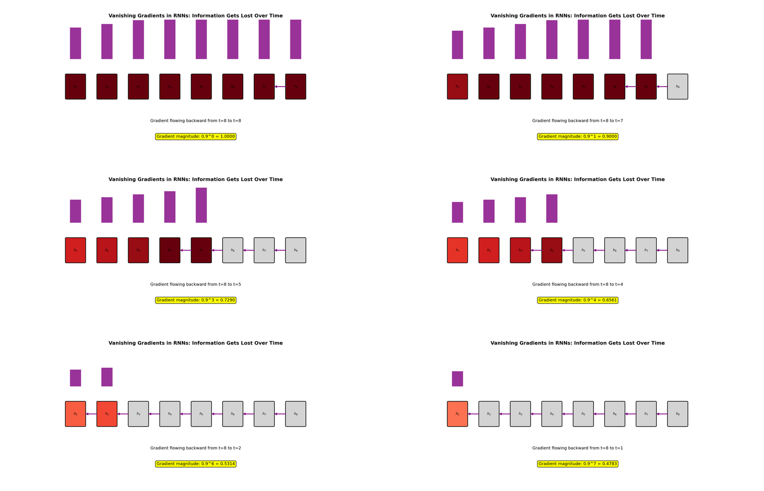
RNNs struggle with long sequences because gradients vanish (or explode) over many timesteps.

Why Gradients Vanish

The gradient from timestep $T$ to timestep $1$:

$$\frac{\partial L_T}{\partial h_1}=\frac{\partial L_T}{\partial h_T}\cdot \prod _{t=2}^T\frac{\partial h_t}{\partial h_{t-1}}$$

Each term $\frac{\partial h_t}{\partial h_{t-1}}=W_{hh}^T\cdot \text{diag}({\tanh }^{\prime }(z_t))$

• If largest eigenvalue of $W_{hh}$ < 1: gradients shrink exponentially
• If largest eigenvalue of $W_{hh}$ > 1: gradients explode

Consequence

Early timesteps receive near-zero gradients — the RNN can't learn long-range dependencies. "The cat [100 words later] was hungry" — RNN forgets about "cat."

---

LSTM: Long Short-Term Memory

LSTMs solve vanishing gradients with a cell state that acts as a highway for gradient flow, controlled by gates.

Architecture

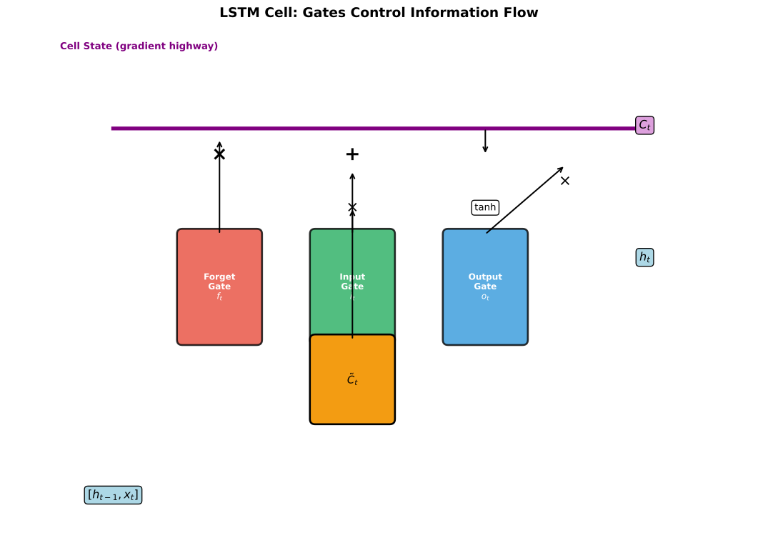
Three gates + cell state:

• Forget gate $f_t$: What to discard from cell state
• Input gate $i_t$: What new information to add
• Output gate $o_t$: What to expose to the next layer

LSTM Equations

Forget gate (what to forget):

$$f_t=\sigma (W_f\cdot [h_{t-1},x_t]+b_f)$$

Input gate (what to update):

$$i_t=\sigma (W_i\cdot [h_{t-1},x_t]+b_i)$$

Candidate values (new information):

$${\tilde{C}}_t=\tanh (W_C\cdot [h_{t-1},x_t]+b_C)$$

Cell state update:

$$C_t=f_t\odot C_{t-1}+i_t\odot {\tilde{C}}_t$$

Output gate (what to expose):

$$o_t=\sigma (W_o\cdot [h_{t-1},x_t]+b_o)$$

Hidden state:

$$h_t=o_t\odot \tanh (C_t)$$

Why LSTM Solves Vanishing Gradients

The cell state update is additive:

$$C_t=f_t\odot C_{t-1}+i_t\odot {\tilde{C}}_t$$

Gradient through cell state:

$$\frac{\partial C_t}{\partial C_{t-1}}=f_t$$

If $f_t\approx 1$ (forget gate open), gradients flow unchanged through many timesteps — the cell state acts as a gradient highway.

---

GRU: Gated Recurrent Unit

GRU simplifies LSTM with 2 gates instead of 3, and no separate cell state.

Architecture

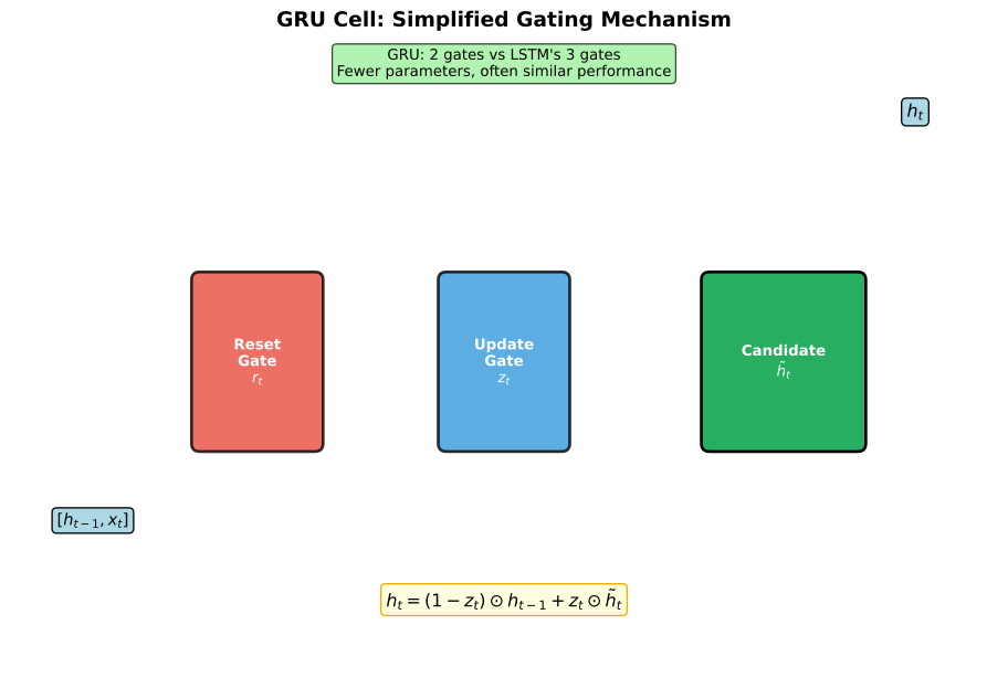
Reset gate (how much past to forget):

$$r_t=\sigma (W_r\cdot [h_{t-1},x_t])$$

Update gate (how much to update):

$$z_t=\sigma (W_z\cdot [h_{t-1},x_t])$$

Candidate hidden state:

$${\tilde{h}}_t=\tanh (W\cdot [r_t\odot h_{t-1},x_t])$$

Final hidden state:

$$h_t=(1-z_t)\odot h_{t-1}+z_t\odot {\tilde{h}}_t$$

LSTM vs GRU

Aspect	LSTM	GRU
Gates	3 (forget, input, output)	2 (reset, update)
States	Cell state + hidden state	Hidden state only
Parameters	More (~4x hidden²)	Fewer (~3x hidden²)
Performance	Often better for complex sequences	Comparable, sometimes better
Training speed	Slower	Faster

Rule of thumb: Start with GRU (faster), try LSTM if GRU underperforms.

---

Bidirectional RNNs

Process sequence in both directions to capture future context:

Forward:   h₁ → h₂ → h₃ → ... → hₜ
Backward:  h₁ ← h₂ ← h₃ ← ... ← hₜ
Output:    [h₁→;h₁←] [h₂→;h₂←] ...

When Bidirectional Helps

• NLP: Understanding "bank" requires future context ("river bank" vs "bank account")
• Speech: Pronunciation depends on following sounds
• NOT for: Real-time prediction (can't see future)

---

RNNs vs Transformers

Aspect	RNNs	Transformers
Processing	Sequential (can't parallelize)	Parallel (all positions at once)
Complexity	O(T) sequential steps	O(T²) attention, but parallelizable
Long-range	Struggles despite gates	Direct attention to any position
Memory	O(1) hidden state size	O(T) keys/values
Inductive bias	Sequential, local	None (learns from data)

Where RNNs Still Matter

1. Streaming/online: Process tokens one at a time
2. Edge devices: Lower memory than storing all keys/values
3. Very long sequences: Linear complexity vs O(T²) attention
4. Causal modeling: Natural fit for sequential generation

Reality: Transformers have largely replaced RNNs for NLP, but RNNs remain relevant for specific use cases.

---

Implementation Tips

Gradient Clipping

Essential for RNN training:

torch.nn.utils.clip_grad_norm_(model.parameters(), max_norm=1.0)

Packed Sequences

Handle variable-length sequences efficiently:

packed = nn.utils.rnn.pack_padded_sequence(x, lengths, batch_first=True)
output, hidden = rnn(packed)
output, _ = nn.utils.rnn.pad_packed_sequence(output, batch_first=True)

Dropout for RNNs

Apply dropout to non-recurrent connections:

nn.LSTM(input_size, hidden_size, dropout=0.2)  # between layers

---

Interview Questions

Q1: "Explain why LSTMs solve the vanishing gradient problem."

The cell state acts as a gradient highway.

In vanilla RNNs, gradients multiply through $W_{hh}$ at each timestep. If eigenvalues < 1, gradients vanish exponentially.

In LSTMs, the cell state update is additive:

$$C_t=f_t\odot C_{t-1}+i_t\odot {\tilde{C}}_t$$

The gradient through cell state:

$$\frac{\partial C_t}{\partial C_{t-1}}=f_t$$

When $f_t\approx 1$ (forget gate open), gradients pass through unchanged. Over many timesteps:

$$\frac{\partial C_T}{\partial C_1}=\prod _{t=2}^T{f}_t\approx 1$$

Key insight: The forget gate learns which information to preserve, allowing gradients to flow to early timesteps. It's not that gradients can't vanish — but the network can learn to keep them flowing for important information.

Q2: "What's the difference between LSTM and GRU?"

LSTM has 3 gates and separate cell/hidden states:

• Forget gate: What to discard from cell
• Input gate: What new info to add
• Output gate: What to expose as hidden state
• Cell state: Long-term memory (gradient highway)

GRU has 2 gates and only hidden state:

• Reset gate: How much past to forget for candidate
• Update gate: Interpolate between old and new state
• No separate cell state

Practical differences:

• GRU has fewer parameters (3x vs 4x hidden²)
• GRU trains faster
• LSTM may capture more complex dependencies
• Performance is often similar

When to choose:

• Start with GRU (simpler, faster)
• Try LSTM if GRU underperforms
• For very complex sequences, LSTM may be better

Q3: "When would you still use RNNs over Transformers?"

Use RNNs when:

1. Online/streaming processing: Need to process tokens one at a time as they arrive (real-time speech, live transcription). Transformers need all tokens to compute attention.

2. Very long sequences: Transformer attention is O(T²). For sequences of 100K+ tokens, RNNs with O(T) complexity may be more practical. (Though efficient transformers like Longformer exist.)

3. Edge deployment: RNN hidden state is fixed size. Transformers store O(T) keys/values, which grows with sequence length.

4. Causal modeling: RNNs have natural sequential inductive bias, which may help with limited data.

Reality: Transformers dominate most NLP tasks. RNNs are still used in niche applications (streaming, embedded systems) and sometimes combined with transformers (transformer encoders + RNN decoders).

---

Key Takeaways

1. RNNs process sequences with shared weights and hidden state memory.

2. Vanilla RNNs suffer from vanishing gradients — can't learn long-range dependencies.

3. LSTM's cell state is a gradient highway — forget gates control what gradients flow through.

4. GRU is simpler than LSTM (2 gates vs 3) with comparable performance.

5. Bidirectional RNNs capture both past and future context.

6. Transformers have largely replaced RNNs but RNNs remain relevant for streaming and edge applications.