Backpropagation

The algorithm that enables deep learning — efficiently computing gradients through neural networks

---

The Problem: Computing Gradients

To train a neural network with gradient descent, we need gradients of the loss with respect to every weight:

$${\theta }^{new}={\theta }^{old}-\alpha \frac{\partial L}{\partial \theta }$$

The challenge: A network with 1 million weights needs 1 million partial derivatives. How do we compute them efficiently?

Naive Approach: Numerical Gradients

Perturb each weight and measure the change in loss:

$$\frac{\partial L}{\partial w_i}\approx \frac{L(w_i+ϵ)-L(w_i-ϵ)}{2ϵ}$$

Problem: Requires 2 forward passes per weight. For 1M weights, that's 2M forward passes per update — far too slow.

The Solution: Backpropagation

Backpropagation computes all gradients in one forward pass + one backward pass, regardless of network size.

---

Computation Graphs

Neural networks can be represented as directed acyclic graphs (DAGs) where:

• Nodes = operations (add, multiply, activation)
• Edges = data flow

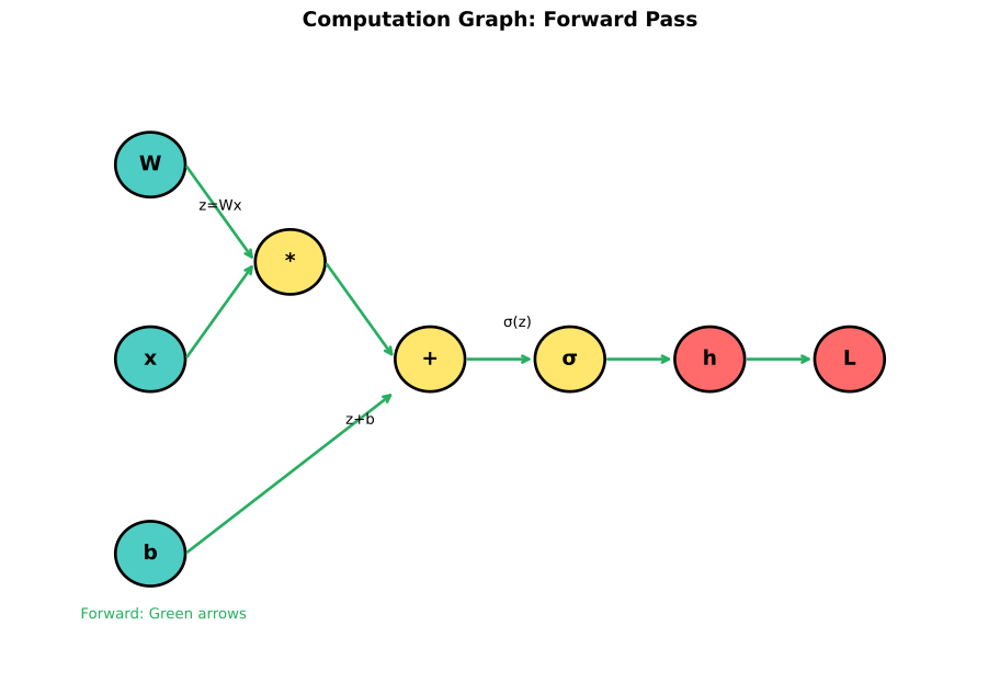
Example: Simple Network

For $y=\sigma (w_2\cdot \sigma (w_1\cdot x+b_1)+b_2)$:

x ──┬──→ [*w₁] ──→ [+b₁] ──→ [σ] ──→ [*w₂] ──→ [+b₂] ──→ [σ] ──→ y
    │                         │
    └─── w₁                   h₁

Each node has:

• Forward: compute output from inputs
• Backward: compute gradient of loss w.r.t. inputs, given gradient w.r.t. output

---

The Chain Rule

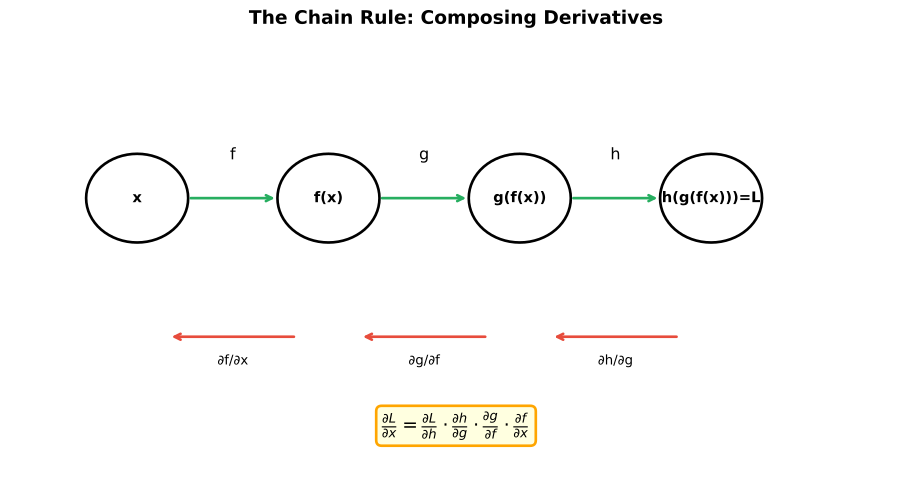
Backpropagation is the chain rule applied systematically through the computation graph.

Single Variable Chain Rule

If $y=f(g(x))$:

$$\frac{dy}{dx}=\frac{dy}{dg}\cdot \frac{dg}{dx}$$

Multivariate Chain Rule

If $L=L(y_1,y_2)$ where $y_1=f_1(x)$ and $y_2=f_2(x)$:

$$\frac{\partial L}{\partial x}=\frac{\partial L}{\partial y_1}\frac{\partial y_1}{\partial x}+\frac{\partial L}{\partial y_2}\frac{\partial y_2}{\partial x}$$

Key insight: Gradients sum when paths merge, and multiply along paths.

---

Backpropagation Algorithm

Forward Pass

Compute activations layer by layer, caching intermediate values:

def forward(x, weights, biases):
    cache = {'a0': x}
    a = x
    for l, (W, b) in enumerate(zip(weights, biases)):
        z = a @ W + b
        cache[f'z{l+1}'] = z
        a = relu(z)  # or other activation
        cache[f'a{l+1}'] = a
    return a, cache

Backward Pass

Propagate gradients from output to input using cached values:

def backward(y_pred, y_true, cache, weights):
    grads = {}
    L = len(weights)

    # Output layer gradient
    dL_da = y_pred - y_true  # for softmax + cross-entropy

    for l in reversed(range(1, L+1)):
        # Gradient through activation
        dL_dz = dL_da * relu_derivative(cache[f'z{l}'])

        # Gradient for weights and biases
        grads[f'dW{l}'] = cache[f'a{l-1}'].T @ dL_dz
        grads[f'db{l}'] = np.sum(dL_dz, axis=0)

        # Propagate to previous layer
        dL_da = dL_dz @ weights[l-1].T

    return grads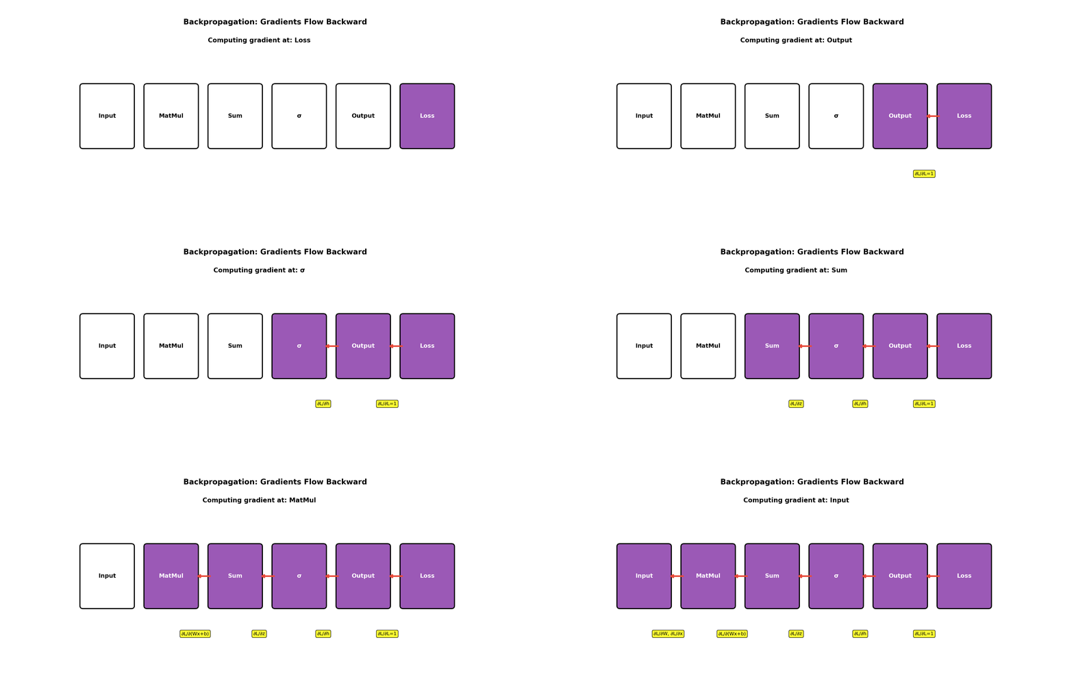

---

Full Derivation: 2-Layer Network

Consider: Input $\mathbf{x}$ → Hidden $\mathbf{h}$ → Output $\hat{\mathbf{y}}$

Forward Pass

$${\mathbf{z}}_1={\mathbf{W}}_1\mathbf{x}+{\mathbf{b}}_1$$$$\mathbf{h}=\sigma ({\mathbf{z}}_1)$$$${\mathbf{z}}_2={\mathbf{W}}_2\mathbf{h}+{\mathbf{b}}_2$$$$\hat{\mathbf{y}}=\text{softmax}({\mathbf{z}}_2)$$

Loss

Cross-entropy: $L=-\sum _i{y}_i\log {\hat{y}}_i$

Backward Pass

Step 1: Output layer gradient (softmax + cross-entropy simplifies nicely)

$$\frac{\partial L}{\partial {\mathbf{z}}_2}=\hat{\mathbf{y}}-\mathbf{y}\equiv {\mathit{\delta }}_2$$

Step 2: Output weight gradients

$$\frac{\partial L}{\partial {\mathbf{W}}_2}={\mathbf{h}}^T{\mathit{\delta }}_2$$$$\frac{\partial L}{\partial {\mathbf{b}}_2}={\mathit{\delta }}_2$$

Step 3: Propagate to hidden layer

$$\frac{\partial L}{\partial \mathbf{h}}={\mathit{\delta }}_2{\mathbf{W}}_2^T$$

Step 4: Through activation

$$\frac{\partial L}{\partial {\mathbf{z}}_1}=\frac{\partial L}{\partial \mathbf{h}}\odot {\sigma }^{\prime }({\mathbf{z}}_1)\equiv {\mathit{\delta }}_1$$

Step 5: Hidden weight gradients

$$\frac{\partial L}{\partial {\mathbf{W}}_1}={\mathbf{x}}^T{\mathit{\delta }}_1$$$$\frac{\partial L}{\partial {\mathbf{b}}_1}={\mathit{\delta }}_1$$

The Pattern

For any layer $l$:

$${\mathit{\delta }}_l={\mathit{\delta }}_{l+1}{\mathbf{W}}_{l+1}^T\odot g^{\prime }({\mathbf{z}}_l)$$$${\mathrm{\nabla }}_{{\mathbf{W}}_l}L={\mathbf{a}}_{l-1}^T{\mathit{\delta }}_l$$

---

Forward Mode vs Reverse Mode Autodiff

Mode	Direction	Efficiency
Forward mode	Input → Output	O(1) for one input, all outputs
Reverse mode	Output → Input	O(1) for one output, all inputs

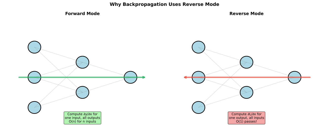
Why Reverse Mode for Neural Networks?

Neural networks have:

• Many inputs (millions of weights)
• One output (scalar loss)

Forward mode: O(n) passes for n weights Reverse mode (backprop): O(1) passes regardless of weight count

---

Implementation Details

Gradient Checking

Verify backprop implementation by comparing to numerical gradients:

def gradient_check(f, x, epsilon=1e-7):
    """Check analytical gradient against numerical gradient."""
    analytical_grad = f.backward(x)
    numerical_grad = np.zeros_like(x)

    for i in range(x.size):
        x_plus = x.copy()
        x_plus.flat[i] += epsilon
        x_minus = x.copy()
        x_minus.flat[i] -= epsilon

        numerical_grad.flat[i] = (f(x_plus) - f(x_minus)) / (2 * epsilon)

    error = np.linalg.norm(analytical_grad - numerical_grad)
    error /= np.linalg.norm(analytical_grad) + np.linalg.norm(numerical_grad)

    return error < 1e-5  # Should be very small

Numerical Stability

Problem: Softmax can overflow for large inputs

Solution: Subtract max before exponentiating

def stable_softmax(z):
    z_shifted = z - np.max(z, axis=-1, keepdims=True)
    exp_z = np.exp(z_shifted)
    return exp_z / np.sum(exp_z, axis=-1, keepdims=True)

Vectorized Implementation

Always work with batches for efficiency:

# Bad: loop over samples
for i in range(batch_size):
    grad_W += x[i:i+1].T @ delta[i:i+1]

# Good: vectorized
grad_W = x.T @ delta  # (input_dim, batch) @ (batch, output_dim)

---

Why Cache Activations?

To compute ${\mathrm{\nabla }}_{{\mathbf{W}}_l}L={\mathbf{a}}_{l-1}^T{\mathit{\delta }}_l$, we need ${\mathbf{a}}_{l-1}$.

Options:

1. Recompute: Run forward pass again (slow)
2. Cache: Store during forward pass (memory-intensive)

Trade-off: Training uses ~2x memory of inference because we cache activations.

Gradient checkpointing: Recompute some activations to trade compute for memory — useful for very large models.

---

Interview Questions

Q1: "Walk through backpropagation for a 2-layer network."

Forward pass:

1. ${\mathbf{z}}_1={\mathbf{W}}_1\mathbf{x}+{\mathbf{b}}_1$ (linear)
2. ${\mathbf{a}}_1=\sigma ({\mathbf{z}}_1)$ (activation)
3. ${\mathbf{z}}_2={\mathbf{W}}_2{\mathbf{a}}_1+{\mathbf{b}}_2$ (linear)
4. $\hat{\mathbf{y}}=\text{softmax}({\mathbf{z}}_2)$ (output)

Loss: $L=-\sum y_i\log {\hat{y}}_i$

Backward pass:

1. ${\mathit{\delta }}_2=\hat{\mathbf{y}}-\mathbf{y}$ (output gradient)
2. ${\mathrm{\nabla }}_{{\mathbf{W}}_2}={\mathbf{a}}_1^T{\mathit{\delta }}_2$ (output weight gradient)
3. ${\mathrm{\nabla }}_{{\mathbf{a}}_1}={\mathit{\delta }}_2{\mathbf{W}}_2^T$ (propagate back)
4. ${\mathit{\delta }}_1={\mathrm{\nabla }}_{{\mathbf{a}}_1}\odot {\sigma }^{\prime }({\mathbf{z}}_1)$ (through activation)
5. ${\mathrm{\nabla }}_{{\mathbf{W}}_1}={\mathbf{x}}^T{\mathit{\delta }}_1$ (hidden weight gradient)

Update: $\mathbf{W}\leftarrow \mathbf{W}-\alpha {\mathrm{\nabla }}_{\mathbf{W}}$

Q2: "Why do we cache activations during forward pass?"

We cache activations because we need them for gradient computation.

The gradient w.r.t. weights at layer $l$ is:

$${\mathrm{\nabla }}_{{\mathbf{W}}_l}L={\mathbf{a}}_{l-1}^T{\mathit{\delta }}_l$$

We need ${\mathbf{a}}_{l-1}$ (the previous layer's activation) to compute this.

Trade-offs:

• Cache everything: Training uses ~2x inference memory
• Recompute: Slower, but saves memory
• Gradient checkpointing: Hybrid — cache some, recompute others

This is why training large models requires much more memory than inference.

Q3: "What's the difference between forward and reverse mode autodiff?"

Forward mode propagates derivatives input → output:

• Efficient for: Few inputs, many outputs
• Complexity: O(n) passes for n inputs

Reverse mode (backpropagation) propagates derivatives output → input:

• Efficient for: Many inputs, few outputs
• Complexity: O(m) passes for m outputs

Neural networks: Millions of weights (inputs to loss), one scalar loss (output). Reverse mode computes all gradients in one backward pass — that's why we use backpropagation.

Forward mode would require millions of passes. The efficiency difference is the reason deep learning is computationally feasible.

---

Key Takeaways

1. Backpropagation is the chain rule applied systematically through a computation graph.

2. Reverse mode autodiff computes all gradients in O(1) backward passes — essential for efficiency.

3. Cache activations during forward pass for use in backward pass (trade memory for speed).

4. Gradient checking validates implementations by comparing to numerical gradients.

5. The pattern: ${\mathit{\delta }}_l={\mathit{\delta }}_{l+1}{\mathbf{W}}_{l+1}^T\odot g^{\prime }({\mathbf{z}}_l)$ — gradients flow backward, multiplying by weights and activation derivatives.