PPO & Modern Policy Optimization

The industry standard — stable, sample-efficient policy learning

---

One-Sentence Summary

PPO constrains policy updates using a clipped surrogate objective, achieving TRPO-level stability without the computational overhead of KL-constrained optimization.

---

Why Trust Regions Matter

The Policy Gradient Instability Problem

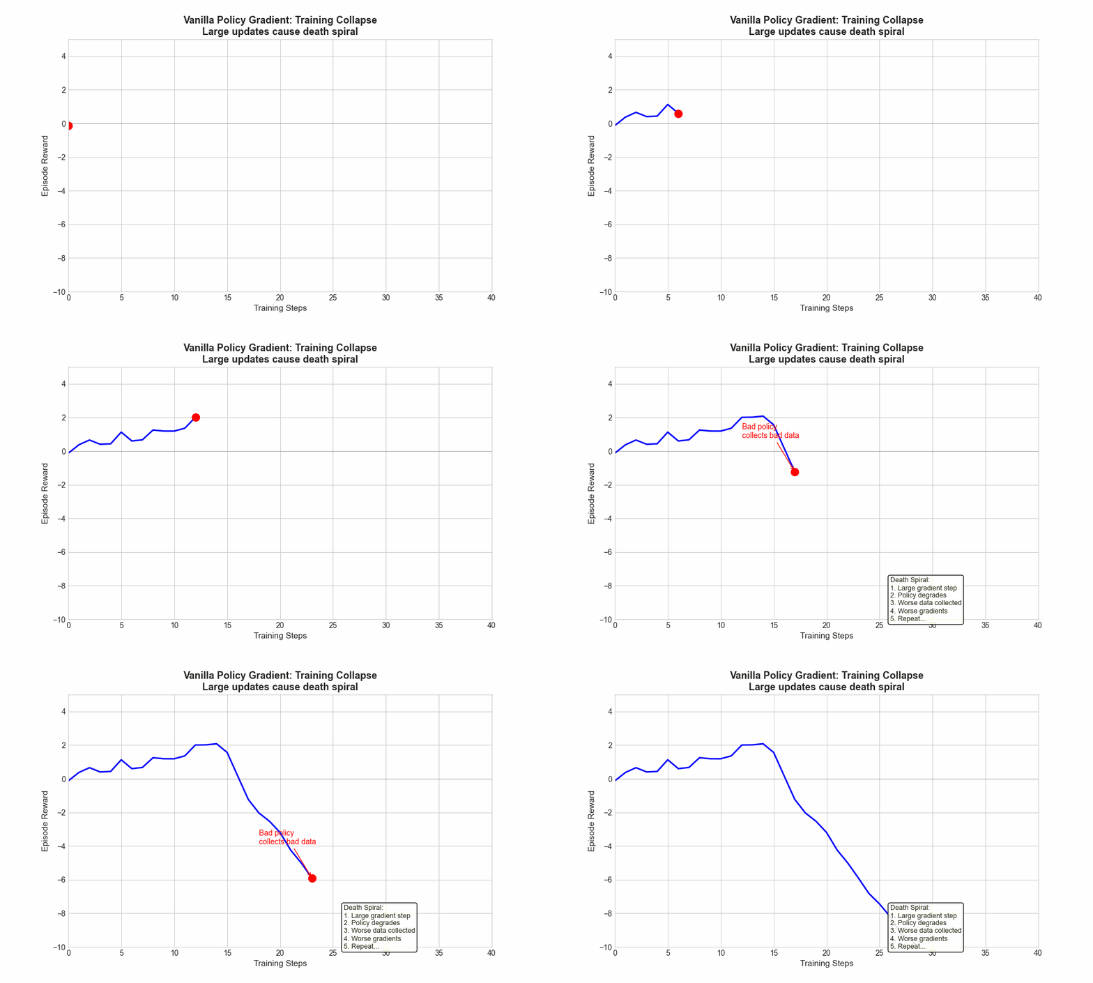
Vanilla policy gradient methods suffer from a critical flaw: unconstrained updates can catastrophically degrade performance.

When we compute the gradient:

$${\mathrm{\nabla }}_{\theta }J(\theta )={\mathbb{E}}_{{\pi }_{\theta }}[{\mathrm{\nabla }}_{\theta }\log {\pi }_{\theta }(a|s)\cdot A^{\pi }(s,a)]$$

A large gradient step can push the policy far from the current distribution. Unlike supervised learning where small errors are recoverable, a bad policy update in RL compounds: the agent collects worse data, which leads to worse gradients, creating a death spiral.

The Trust Region Insight

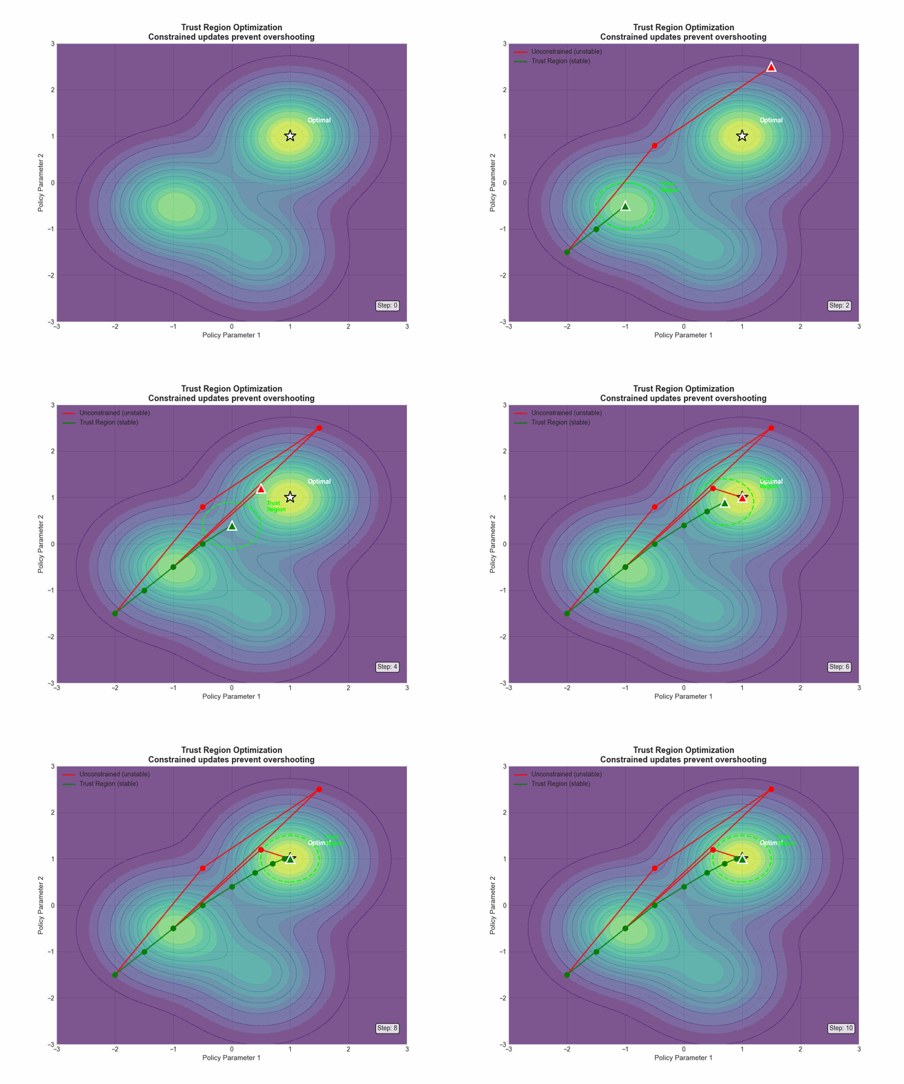
The core insight: limit how much the policy can change per update. If we stay within a "trust region" where our gradient estimates are reliable, training becomes stable.

Mathematically, we want to maximize the expected improvement while constraining policy divergence:

$$\text{maximize }\mathbb{E}[\frac{{\pi }_{\theta }(a|s)}{{\pi }_{{\theta }_{old}}(a|s)}{A}^{{\pi }_{{\theta }_{old}}}(s,a)]$$$$\text{subject to }{D}_{KL}({\pi }_{{\theta }_{old}}\parallel {\pi }_{\theta })\le \delta$$

This is the foundation of modern policy optimization.

---

TRPO: Trust Region Policy Optimization

The KL-Constrained Objective

TRPO (Schulman et al., 2015) formalizes the trust region idea using KL divergence as the constraint:

$$\text{maximize }\mathcal{L}(\theta )={\mathbb{E}}_t[r_t(\theta ){\hat{A}}_t]$$$$\text{subject to }{\mathbb{E}}_t[D_{KL}({\pi }_{{\theta }_{old}}(\cdot |s_t)\parallel {\pi }_{\theta }(\cdot |s_t))]\le \delta$$

Where the probability ratio is:

$$r_t(\theta )=\frac{{\pi }_{\theta }(a_t|s_t)}{{\pi }_{{\theta }_{old}}(a_t|s_t)}$$

Why TRPO Works

TRPO guarantees monotonic improvement under certain conditions. The constraint ensures:

1. Bounded distribution shift — new policy stays close to old policy
2. Valid importance sampling — gradient estimates remain accurate
3. Stable training — no catastrophic policy collapse

TRPO's Computational Burden

The problem: solving a constrained optimization requires computing the Fisher Information Matrix and performing conjugate gradient descent for each update.

For each policy update:
    1. Compute policy gradient g
    2. Estimate Fisher matrix F (expensive!)
    3. Solve F^{-1}g using conjugate gradient
    4. Line search to find step size satisfying KL constraint

This is computationally expensive and complex to implement, motivating PPO.

---

PPO: Proximal Policy Optimization

The Clipped Surrogate Objective

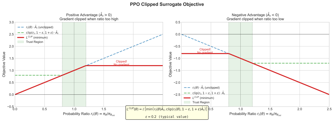
PPO (Schulman et al., 2017) achieves similar stability to TRPO with a remarkably simple change: clip the objective function instead of adding constraints.

The PPO-Clip objective:

$$L^{CLIP}(\theta )={\mathbb{E}}_t[min(r_t(\theta ){\hat{A}}_t,\text{clip}(r_t(\theta ),1-ϵ,1+ϵ){\hat{A}}_t)]$$

Where:

• $r_t(\theta )=\frac{{\pi }_{\theta }(a_t|s_t)}{{\pi }_{{\theta }_{old}}(a_t|s_t)}$ is the probability ratio
• ${\hat{A}}_t$ is the advantage estimate (typically from GAE)
• $ϵ$ is the clipping hyperparameter (typically 0.1-0.2)

How Clipping Provides Trust Regions

The clipping mechanism creates an implicit trust region:

Scenario	$r_t(\theta )$	Effect
Good action ($A_t>0$), ratio too high	$r_t>1+ϵ$	Gradient clipped, prevents over-optimization
Good action ($A_t>0$), ratio in range	$1-ϵ\le r_t\le 1+ϵ$	Normal gradient
Bad action ($A_t<0$), ratio too low	$r_t<1-ϵ$	Gradient clipped, prevents over-correction
Bad action ($A_t<0$), ratio in range	$1-ϵ\le r_t\le 1+ϵ$	Normal gradient

The minimum in the objective ensures:

• For positive advantages: we clip when the ratio exceeds $1+ϵ$
• For negative advantages: we clip when the ratio drops below $1-ϵ$

This prevents the policy from moving too far in either direction.

PPO in Practice

The full PPO objective includes additional terms:

$$L(\theta )=L^{CLIP}(\theta )-c_1{L}^{VF}(\theta )+c_{2}S[{\pi }_{\theta }](s_t)$$

Where:

• $L^{VF}$ is the value function loss (for actor-critic)
• $S[{\pi }_{\theta }]$ is an entropy bonus for exploration
• $c_1,c_2$ are coefficients (typically $c_1=0.5$, $c_2=0.01$)

Key hyperparameters:

Parameter	Typical Value	Purpose
$ϵ$ (clip range)	0.1 - 0.2	Trust region size
Learning rate	$3\times {10}^{-4}$	Step size
GAE $\lambda$	0.95	Advantage estimation bias-variance
Epochs per batch	3-10	Number of passes over collected data
Mini-batch size	64-4096	Batch size for gradient updates

---

Why PPO is the Industry Standard

Simplicity + Performance

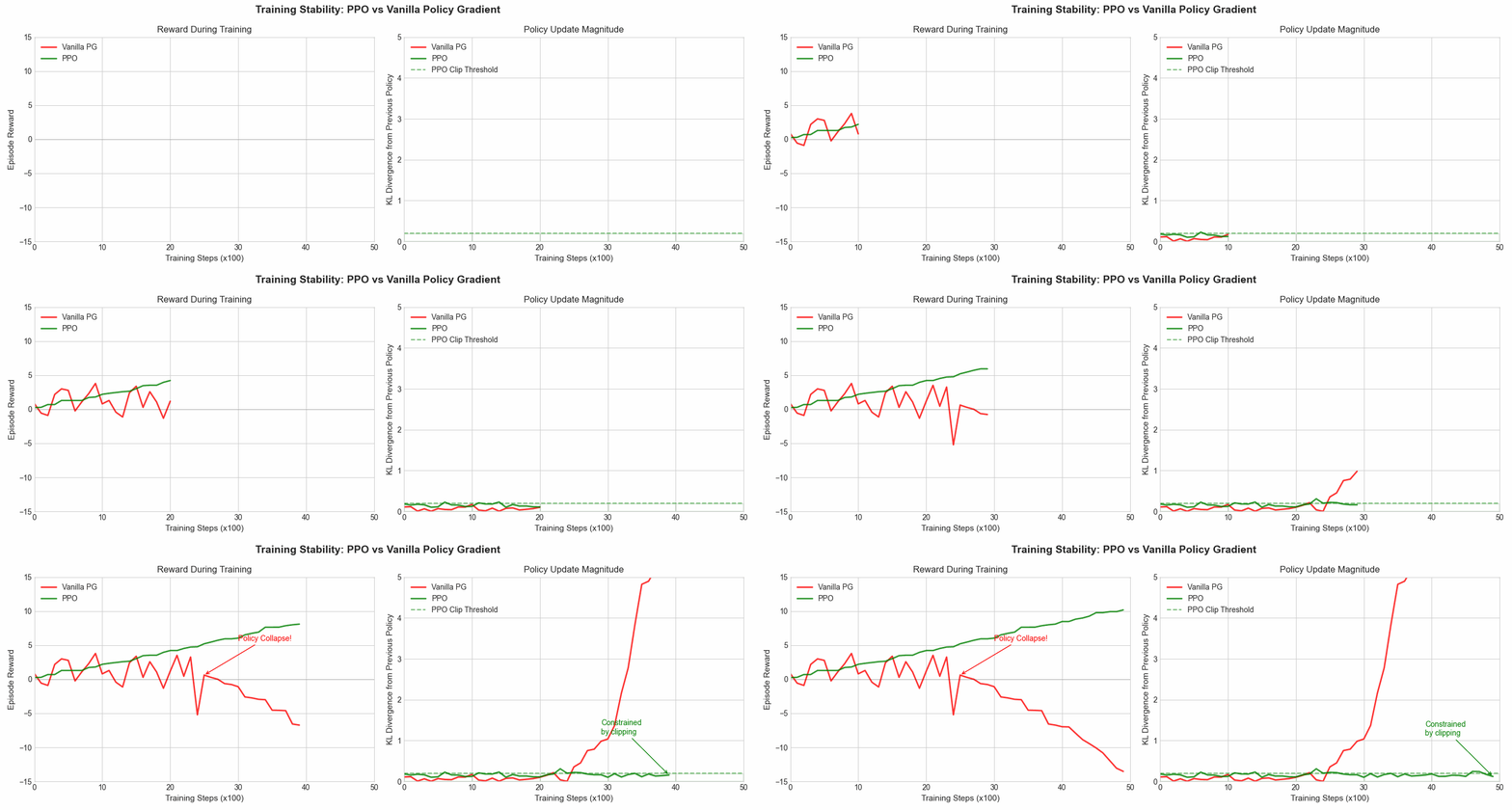
PPO dominates practical RL for several reasons:

1. Simple implementation — just a few lines of clipping code
2. First-order optimization — standard gradient descent, no Hessian/Fisher
3. Sample efficiency — multiple epochs over collected data
4. Robust to hyperparameters — works well with default settings
5. Parallelizable — easy to scale across workers

Industry Adoption

PPO (or variants) powers:

• OpenAI Five — Dota 2 AI
• ChatGPT RLHF — language model alignment
• Robotics — manipulation and locomotion
• Game AI — Atari, continuous control benchmarks

When to Use PPO

Use Case	Recommendation
General continuous control	PPO (default choice)
Discrete action spaces	PPO works well
RLHF / LLM training	PPO (standard approach)
High-dimensional observations	PPO + CNN/Transformer
Offline RL	Consider other methods (CQL, IQL)
Maximum sample efficiency needed	SAC may be better

---

SAC: Soft Actor-Critic

Maximum Entropy RL

SAC (Haarnoja et al., 2018) takes a different approach: instead of constraining policy updates, it encourages exploration through an entropy bonus.

The SAC objective maximizes expected return plus entropy:

$$J(\pi )=\sum _{t=0}^T{\mathbb{E}}_{(s_t,a_t)\sim {\rho }_{\pi }}[r(s_t,a_t)+\alpha \mathcal{H}(\pi (\cdot |s_t))]$$

Where $\mathcal{H}(\pi (\cdot |s_t))=-{\mathbb{E}}_{a\sim \pi }[\log \pi (a|s_t)]$ is the policy entropy.

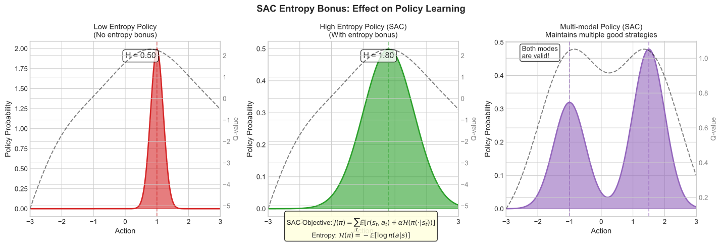
Why Entropy Matters

The entropy bonus has profound effects:

1. Exploration — high-entropy policies try diverse actions
2. Robustness — stochastic policies are less brittle
3. Multi-modality — can maintain multiple good behaviors
4. Stability — prevents premature convergence to deterministic policies

SAC Architecture

SAC is an off-policy actor-critic method with:

• Two Q-networks (for double Q-learning, reduces overestimation)
• One policy network (outputs mean and std of Gaussian)
• Automatic temperature tuning ($\alpha$ learned to hit target entropy)

SAC vs PPO

Aspect	PPO	SAC
On/Off-policy	On-policy	Off-policy
Sample efficiency	Lower	Higher
Stability	Very stable	Stable
Exploration	Entropy bonus (optional)	Core mechanism
Continuous actions	Supported	Designed for
Discrete actions	Native support	Requires modification
Implementation	Simple	Moderate

---

Algorithm Selection Guide

Quick Decision Matrix

Scenario	Best Choice	Why
RLHF for LLMs	PPO	Standard, well-tested
Robotics sim-to-real	SAC	Sample efficiency
Game AI (discrete)	PPO	Native discrete support
Continuous control benchmark	SAC/TD3	Higher final performance
First RL project	PPO	Simplicity, robustness
Real robot (limited samples)	SAC	Off-policy efficiency

---

Interview Questions

Q1: "Explain why PPO uses clipping instead of a KL constraint like TRPO."

"TRPO enforces a hard KL divergence constraint, which requires expensive second-order optimization — computing the Fisher information matrix and using conjugate gradient descent for each update.

PPO achieves similar stability through a much simpler mechanism: clipping the probability ratio. The clipped objective:

$$L^{CLIP}(\theta )=\mathbb{E}[min(r_t(\theta ){\hat{A}}_t,\text{clip}(r_t(\theta ),1-ϵ,1+ϵ){\hat{A}}_t)]$$

When the ratio $r_t$ moves outside $[1-ϵ,1+ϵ]$, the gradient becomes zero — this implicitly creates a trust region. The key insight is that clipping is a first-order operation requiring only standard gradient descent, making PPO orders of magnitude faster to compute while maintaining similar stability guarantees.

Empirically, PPO matches or exceeds TRPO performance on most benchmarks while being much simpler to implement and tune."

Q2: "Why does SAC include an entropy bonus, and how does it differ from PPO's exploration strategy?"

"SAC uses entropy maximization as a core objective, not just for exploration but as part of the fundamental optimization goal:

$$J(\pi )=\mathbb{E}[\sum _t{r}_t+\alpha \mathcal{H}(\pi (\cdot |s_t))]$$

This has several effects:

1. Principled exploration: High entropy means trying diverse actions proportional to their Q-values
2. Robustness: Stochastic policies handle uncertainty better than deterministic ones
3. Multi-modality: The policy can maintain multiple good solutions rather than collapsing to one

PPO's exploration is typically more ad-hoc — adding a small entropy bonus ($c_{2}S[\pi ]$) to prevent premature convergence, but it's not central to the algorithm.

The key difference: SAC is off-policy (uses replay buffer), so the entropy bonus helps ensure continued exploration of the state space. PPO is on-policy (discards old data), so exploration comes naturally from collecting new trajectories with the current policy."

Q3: "When would you choose SAC over PPO for a production system?"

"I'd choose SAC over PPO in these scenarios:

1. Sample efficiency is critical: SAC is off-policy and can reuse experience from a replay buffer. If each environment interaction is expensive (real robots, expensive simulations), SAC's 2-5x better sample efficiency matters.

2. Continuous action spaces: SAC was specifically designed for continuous control with Gaussian policies. While PPO handles continuous actions, SAC often achieves higher asymptotic performance.

3. Need for exploration in sparse rewards: SAC's entropy maximization provides principled exploration even without reward shaping.

I'd stick with PPO when:

• Actions are discrete (SAC requires modifications)
• Implementation simplicity is paramount
• Using RLHF for language models (established practice)
• Parallelization across many workers is needed (on-policy scales better)

Practical note: For most problems, try PPO first. Switch to SAC if sample efficiency becomes a bottleneck or if you need better final performance on continuous control tasks."

---

Quick Reference Card

PPO ESSENTIALS
---------------------------------------------------
Objective:   L^CLIP = E[min(r_t * A_t, clip(r_t, 1-e, 1+e) * A_t)]
Ratio:       r_t = pi_new(a|s) / pi_old(a|s)
Clip range:  epsilon = 0.1 - 0.2
Key insight: Clipping = implicit trust region

ALGORITHM COMPARISON
---------------------------------------------------
           | PPO         | SAC         | TRPO
-----------+-------------+-------------+------------
Policy     | On-policy   | Off-policy  | On-policy
Stability  | Very high   | High        | Very high
Efficiency | Medium      | High        | Medium
Complexity | Simple      | Medium      | Complex
Actions    | Any         | Continuous  | Any

SAC ESSENTIALS
---------------------------------------------------
Objective:  J = E[sum(r_t + alpha * H(pi))]
Entropy:    H(pi) = -E[log pi(a|s)]
Key insight: Entropy bonus enables robust exploration

HYPERPARAMETERS (PPO)
---------------------------------------------------
Clip epsilon:    0.1 - 0.2
Learning rate:   3e-4
GAE lambda:      0.95
Epochs/batch:    3 - 10
Entropy coeff:   0.01

WHEN TO USE WHAT
---------------------------------------------------
PPO:  Default choice, discrete actions, RLHF, simplicity
SAC:  Sample efficiency, continuous control, robotics
TRPO: When you need formal guarantees (rare in practice)

---

Key Takeaways

1. Trust regions prevent catastrophic policy updates — constraining how much the policy can change per update ensures stable training and prevents death spirals.

2. PPO's clipped objective is brilliantly simple — instead of solving constrained optimization like TRPO, clipping the probability ratio achieves similar stability with first-order gradients only.

3. The probability ratio $r_t(\theta )$ is the key quantity — it measures how much the new policy differs from the old policy for each action, enabling importance sampling and stability control.

4. SAC trades complexity for sample efficiency — by being off-policy with entropy maximization, SAC can achieve better performance with fewer environment interactions.

5. PPO is the industry default for good reason — simple, stable, parallelizable, and effective across discrete and continuous domains. Start here unless you have specific reasons to choose otherwise.