Exploration vs Exploitation

The fundamental trade-off in RL — when to try new things vs stick with what works

---

The Core Dilemma

Every learning agent faces a fundamental question: should I exploit my current best option, or explore to potentially find something better?

• Exploitation: Select the action that appears best based on current knowledge
• Exploration: Try different actions to improve knowledge of their rewards

The key insight: pure exploitation converges to a suboptimal policy if the best action was never discovered; pure exploration wastes resources gathering information never used.

---

Multi-Armed Bandit: The Canonical Problem

Problem Setup

Imagine $K$ slot machines (arms), each with unknown reward distribution $R_a$. At each timestep $t$:

1. Select an arm $a_t\in \{1,2,...,K\}$
2. Receive reward $r_t\sim R_{a_t}$
3. Update knowledge about arm $a_t$

Goal: Maximize cumulative reward over $T$ timesteps.

The true mean reward for arm $a$ is ${\mu }_a=\mathbb{E}[R_a]$. The optimal arm is $a^{\ast }=\arg \underset{a}{max}{\mu }_a$.

Estimating Arm Values

After $n_a(t)$ pulls of arm $a$, we estimate its value:

$${\hat{Q}}_t(a)=\frac{1}{n_a(t)}\sum _{i=1}^t{r}_i\cdot \mathbb{1}[a_i=a]$$

This is simply the sample mean of observed rewards for arm $a$.

---

Exploration Strategies

1. Epsilon-Greedy

The simplest approach: with probability $ϵ$, explore randomly; otherwise, exploit.

$$a_t=\{\begin{array}{ll}\arg \underset{a}{max}{\hat{Q}}_t(a)& \text{with probability }1-ϵ\\ \text{random arm}& \text{with probability }ϵ\end{array}$$

Advantages: Simple, guarantees exploration Disadvantages: Explores uniformly (even clearly bad arms), fixed exploration rate

Decay Schedules

Fixed $ϵ$ is suboptimal. As we gather more data, we should explore less:

Schedule	Formula	Properties
Linear decay	${ϵ}_t=max({ϵ}_{min},{ϵ}_0-t/T)$	Predictable, may decay too fast
Exponential decay	${ϵ}_t={ϵ}_0\cdot {\gamma }^t$	Common in deep RL
Inverse time	${ϵ}_t={ϵ}_0/(1+t/T)$	Slower decay, theoretically motivated

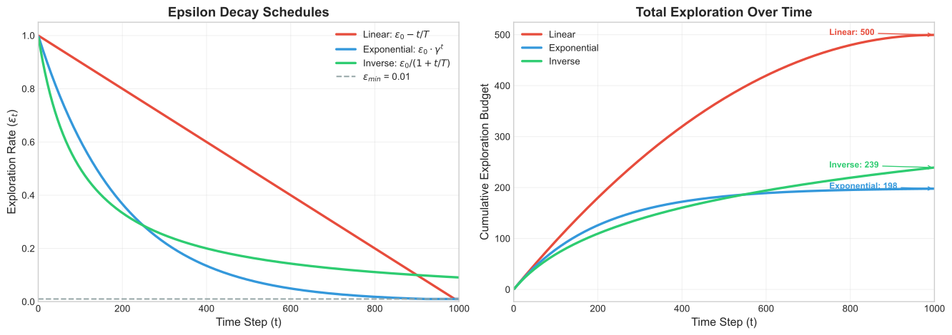
Interview insight: The optimal decay rate depends on the problem horizon $T$ and the gap between arm values.

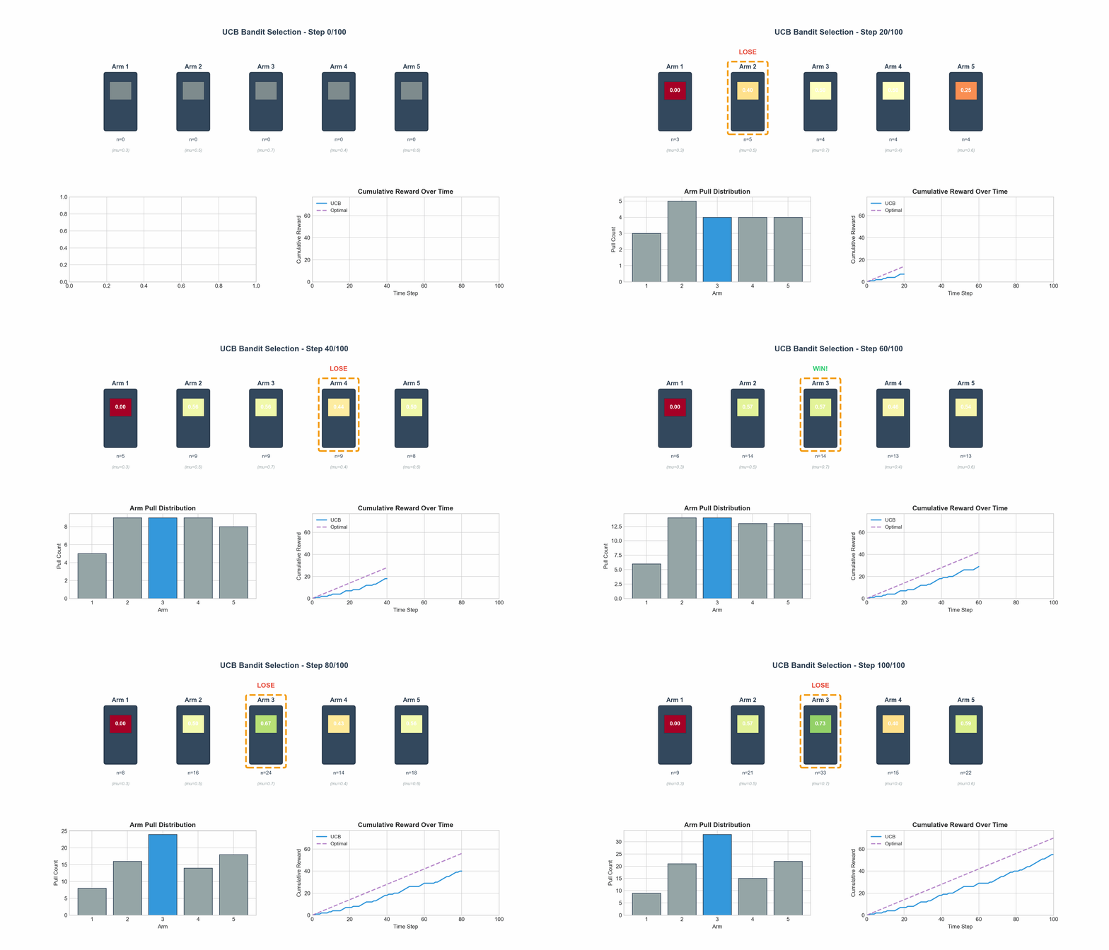
2. Upper Confidence Bound (UCB)

UCB addresses a key limitation of $ϵ$-greedy: it treats all uncertain arms equally. Instead, UCB balances the estimated value with uncertainty:

$$a_t=\arg \underset{a}{max}[{\hat{Q}}_t(a)+c\sqrt{\frac{\ln t}{n_a(t)}}]$$

The second term is the exploration bonus:

• Large when arm $a$ has been pulled rarely ($n_a(t)$ small)
• Shrinks as we pull arm $a$ more often
• Grows slowly with total timesteps $t$ (via $\ln t$)

Intuition: UCB implements "optimism in the face of uncertainty" — it assumes uncertain arms might be good until proven otherwise.

Why $\ln t$? This ensures the exploration bonus grows sublogarithmically, achieving optimal regret bounds.

3. Thompson Sampling

Thompson Sampling takes a Bayesian approach: maintain a probability distribution over each arm's mean, then sample from these posteriors.

Algorithm:

1. For each arm $a$, maintain posterior $P({\mu }_a|\text{data})$
2. Sample ${\tilde{\mu }}_a\sim P({\mu }_a|\text{data})$ for each arm
3. Select $a_t=\arg \underset{a}{max}{\tilde{\mu }}_a$

For Bernoulli bandits (binary rewards), we use Beta distributions:

$${\mu }_a|\text{data}\sim \text{Beta}({\alpha }_a+{\text{successes}}_a,{\beta }_a+{\text{failures}}_a)$$

Advantages:

• Naturally balances exploration/exploitation through posterior sampling
• Often outperforms UCB in practice
• Easily extends to contextual bandits

Disadvantages:

• Requires specifying priors
• Posterior may be intractable for complex reward models

Strategy Comparison

Strategy	Exploration Type	Regret Bound	Computational Cost
$ϵ$-greedy	Uniform random	$O(ϵT+K/ϵ)$	$O(K)$
UCB	Uncertainty-driven	$O(\sqrt{KT\ln T})$	$O(K)$
Thompson Sampling	Posterior sampling	$O(\sqrt{KT\ln T})$	$O(K)$ per sample

---

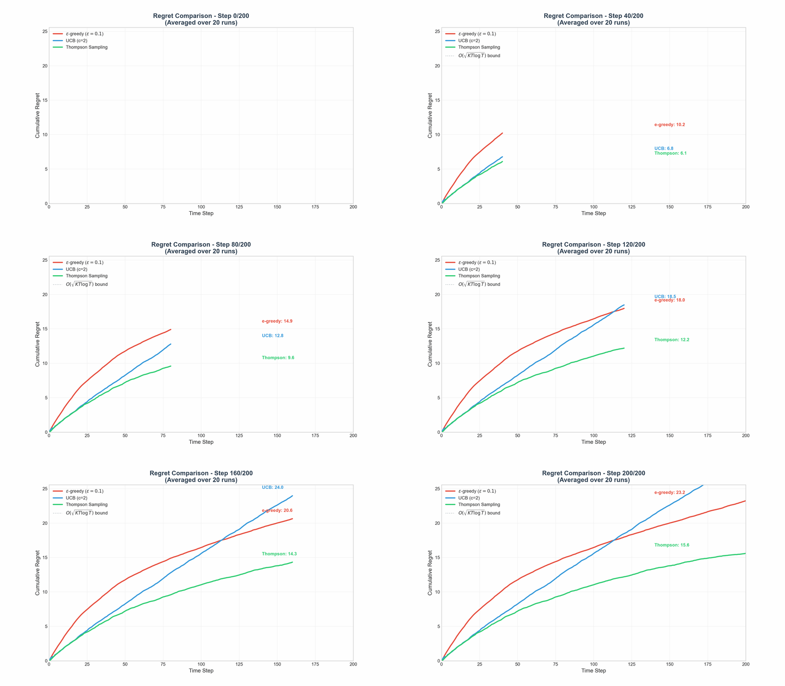
Regret: Measuring Performance

Definition

Regret quantifies the cost of learning — the cumulative difference between the optimal policy and our chosen actions:

$$\text{Regret}(T)=\sum _{t=1}^T({\mu }^{\ast }-{\mu }_{a_t})=T{\mu }^{\ast }-\sum _{t=1}^T{\mu }_{a_t}$$

where ${\mu }^{\ast }=\underset{a}{max}{\mu }_a$ is the optimal arm's mean reward.

Regret Bounds

Lower bound (Lai-Robbins): Any consistent algorithm must have:

$$\underset{T\to \mathrm{\infty }}{lim inf}\frac{\text{Regret}(T)}{\ln T}\ge \sum _{a:{\mu }_a<{\mu }^{\ast }}\frac{{\mu }^{\ast }-{\mu }_a}{\text{KL}({\mu }_a||{\mu }^{\ast })}$$

This establishes that $O(\ln T)$ regret is the best possible for problem-dependent bounds.

Problem-independent bounds: UCB and Thompson Sampling achieve:

$$\text{Regret}(T)=O(\sqrt{KT\ln T})$$

This scales with the square root of time — sublinear growth means we're learning effectively.

Interpreting Regret

Regret Growth	Interpretation
$O(T)$	Linear — not learning (pure exploration)
$O(\sqrt{T})$	Sublinear — effective learning
$O(\ln T)$	Logarithmic — near-optimal

---

Extension to Full MDPs

The bandit problem is a special case of MDPs with a single state. In full MDPs:

The Exploration Challenge

States compound the exploration problem:

• Must explore actions at each state
• Must explore states themselves (may need specific action sequences)
• Rewards may be sparse and delayed

Exploration Methods in MDPs

1. Epsilon-greedy policy: Same principle, applied to Q-learning or policy gradient

$$\pi (a|s)=\{\begin{array}{ll}1-ϵ+\frac{ϵ}{|A|}& \text{if }a=\arg \underset{a^{\prime }}{max}Q(s,a^{\prime })\\ \frac{ϵ}{|A|}& \text{otherwise}\end{array}$$

2. UCB for MDPs (UCRL, UCB-VI): Maintain confidence bounds on transition probabilities and rewards, then plan optimistically.

3. Intrinsic motivation: Add exploration bonuses to rewards:

$$r_t^{\text{total}}=r_t^{\text{extrinsic}}+\beta \cdot r_t^{\text{intrinsic}}$$

Common intrinsic rewards:

• Count-based: $r^{\text{intrinsic}}(s)=1/\sqrt{n(s)}$ (bonus for visiting rare states)
• Prediction error: Reward proportional to model's surprise
• Information gain: Reward for reducing uncertainty about dynamics

4. Posterior sampling for RL (PSRL): Thompson Sampling extended to MDPs — sample a complete MDP from the posterior and act optimally in it.

---

Interview Questions

Question 1: Explain the exploration-exploitation trade-off. Why can't we just exploit?

Expected Answer:

"Pure exploitation fails because initial estimates may be inaccurate. If the true best arm was unlucky in early samples, we might never discover it.

Consider two arms with true means ${\mu }_1=0.6$ and ${\mu }_2=0.8$. If arm 1 gets lucky and returns 1.0 first while arm 2 returns 0.5, pure exploitation locks onto arm 1 forever, accumulating linear regret.

Different strategies balance this: $ϵ$-greedy adds random exploration, UCB explores uncertain options, and Thompson Sampling samples from posteriors."

---

Question 2: Compare UCB and Thompson Sampling. When would you prefer one over the other?

Expected Answer:

"Both achieve optimal $O(\sqrt{KT\ln T})$ regret bounds but differ in approach:

UCB: Deterministic, explicit exploration bonus ($c\sqrt{\ln t/n_a}$), easier to analyze, requires tuning $c$.

Thompson Sampling: Stochastic via posterior sampling, often better empirically, requires specifying priors.

Choose UCB for deterministic/reproducible behavior or when theoretical guarantees matter. Choose Thompson Sampling for better empirical performance, especially in production systems like ad recommendation."

---

Question 3: How does exploration differ between bandits and full MDPs? What additional challenges arise?

Expected Answer:

"In bandits, exploration is about trying different actions. In MDPs, this is compounded by:

1. State space exploration: Some states require specific action sequences to reach
2. Credit assignment: Rewards may be delayed by many timesteps
3. Compounding errors: Bad states lead to many suboptimal timesteps
4. Curse of dimensionality: Count-based exploration fails in large state spaces

Solutions: Intrinsic motivation (curiosity bonuses), optimistic initialization, model-based exploration, hierarchical methods. The key insight is that MDPs require exploring the state-action space, not just actions."

---

Quick Reference Card

+------------------------------------------------------------------+
|              EXPLORATION VS EXPLOITATION CHEAT SHEET              |
+------------------------------------------------------------------+

CORE TRADE-OFF
  Exploit: Use current best action (greedy)
  Explore: Try other actions (information gathering)

MULTI-ARMED BANDIT
  K arms, unknown reward distributions
  Goal: Maximize sum of rewards over T pulls
  Optimal arm: a* = argmax_a mu_a

STRATEGIES
  +------------------+---------------------------+------------------+
  | Strategy         | Selection Rule            | Regret Bound     |
  +------------------+---------------------------+------------------+
  | epsilon-greedy   | Random w.p. epsilon       | O(T) or better   |
  | UCB              | Q(a) + c*sqrt(ln(t)/n_a)  | O(sqrt(KT ln T)) |
  | Thompson         | Sample from posteriors    | O(sqrt(KT ln T)) |
  +------------------+---------------------------+------------------+

REGRET DEFINITION
  Regret(T) = T*mu* - sum_{t=1}^T mu_{a_t}

  Lower bound: Omega(ln T) problem-dependent
  Optimal: O(sqrt(KT ln T)) problem-independent

UCB FORMULA
  a_t = argmax_a [ Q(a) + c * sqrt(ln(t) / n_a(t)) ]
                   ^^^^^   ^^^^^^^^^^^^^^^^^^^^^^^^^
                   exploit        explore

THOMPSON SAMPLING (Bernoulli)
  Prior: Beta(alpha, beta)
  Posterior: Beta(alpha + successes, beta + failures)
  Select: argmax_a sample_a

EPSILON DECAY SCHEDULES
  Linear:      epsilon_t = max(eps_min, eps_0 - t/T)
  Exponential: epsilon_t = eps_0 * gamma^t
  Inverse:     epsilon_t = eps_0 / (1 + t/T)

MDP EXPLORATION
  Challenge: Must explore states AND actions
  Solutions: Intrinsic rewards, optimistic init, PSRL

  Intrinsic reward examples:
    - Count-based: 1/sqrt(n(s))
    - Prediction error (curiosity)
    - Information gain

KEY INSIGHTS FOR INTERVIEWS
  1. Pure exploitation: O(T) regret (linear = bad)
  2. Pure exploration: O(T) regret (linear = bad)
  3. Good algorithms: O(sqrt(T)) or O(ln T) regret
  4. UCB: Optimism in face of uncertainty
  5. Thompson: Probability matching via posteriors

+------------------------------------------------------------------+

---

Key Takeaways

1. Exploration-exploitation is universal: Any learning system must balance gathering information with using it optimally.

2. Regret quantifies learning efficiency: Sublinear regret ($o(T)$) means we're converging to optimal behavior.

3. UCB implements optimism: By adding uncertainty bonuses, UCB naturally explores under-sampled options while favoring high-value ones.

4. Thompson Sampling often wins empirically: Despite similar theoretical guarantees to UCB, Thompson Sampling typically performs better in practice.

5. MDPs compound the exploration challenge: State visitation, delayed rewards, and large state spaces require sophisticated exploration strategies beyond simple bandit algorithms.

6. Decay schedules matter: In finite-horizon problems, exploration should decrease over time as we become more confident in our estimates.

Understanding these concepts is essential for designing effective RL systems and for interview success — these questions probe your understanding of fundamental RL principles that underlie everything from recommendation systems to robotics.