Vanishing and Exploding Gradients Interview FAQ

Understand and solve gradient flow problems

Gradient flow problems are among the most critical challenges in training deep neural networks. This FAQ covers the causes, diagnosis, and solutions for vanishing and exploding gradients - essential knowledge for any machine learning interview.

---

Fundamentals

Q1: What is the vanishing gradient problem?

Answer: The vanishing gradient problem occurs when gradients become exponentially small as they propagate backward through many layers of a neural network. This causes earlier layers to learn extremely slowly or not at all.

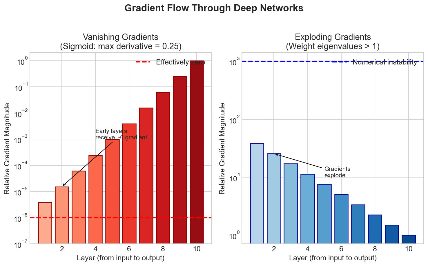
Mathematical Explanation:

During backpropagation, gradients are computed using the chain rule:

∂L/∂W₁ = ∂L/∂aₙ × ∂aₙ/∂aₙ₋₁ × ... × ∂a₂/∂a₁ × ∂a₁/∂W₁

If each partial derivative is less than 1 (e.g., sigmoid's max of 0.25), gradients decay exponentially. After 10 layers with factor 0.25: gradient becomes ~10⁻⁶ (effectively zero).

Consequences: Early layers receive near-zero gradients, weights barely update, and training plateaus.

---

Q2: What is the exploding gradient problem?

Answer: The exploding gradient problem is the opposite - gradients grow exponentially large as they propagate backward, causing unstable training and numerical overflow.

Mathematical Explanation:

If gradient terms are greater than 1 (e.g., 2.0):

• After 10 layers: 2¹⁰ = 1024
• After 20 layers: 2²⁰ ≈ 1,000,000

Symptoms:

• Loss becomes NaN or infinity
• Weights grow to very large values
• Model predictions become unstable
• Training diverges completely

Example Code Demonstrating the Problem:

import numpy as np

def simulate_gradient_flow(num_layers, gradient_factor):
    """Simulate gradient magnitude through layers."""
    gradient = 1.0
    for layer in range(num_layers):
        gradient *= gradient_factor
    return gradient

# Vanishing: factor < 1
print(f"Vanishing (50 layers, factor=0.5): {simulate_gradient_flow(50, 0.5):.2e}")
# Output: 8.88e-16

# Exploding: factor > 1
print(f"Exploding (50 layers, factor=1.5): {simulate_gradient_flow(50, 1.5):.2e}")
# Output: 6.38e+08

---

Q3: What are the main causes of vanishing gradients?

Answer: Several factors contribute to vanishing gradients:

1. Saturating Activation Functions:

• Sigmoid: derivative max = 0.25, tanh: max = 1.0
• When inputs are large, derivatives approach 0 (saturation)

2. Poor Weight Initialization:

• Weights initialized too small multiply gradients toward zero

3. Deep Networks:

• More layers = more gradient multiplications, compounding decay

4. Recurrent Neural Networks:

• Same weights applied repeatedly across time steps

---

Q4: What are the main causes of exploding gradients?

Answer: Exploding gradients typically result from:

1. Poor Weight Initialization:

• Weights initialized too large amplify gradients
• Each layer multiplies the gradient by weight matrices

2. Deep Networks with Amplifying Gradients:

• If weight matrices have eigenvalues > 1
• Gradients grow exponentially through layers

3. Recurrent Neural Networks:

• Particularly problematic for long sequences
• Same weight matrix applied repeatedly

4. High Learning Rates:

• Large weight updates can push activations into extreme regions
• Creates a feedback loop of increasingly large gradients

Example - Weight Matrix Eigenvalues:

import numpy as np

# Weight matrix with eigenvalues > 1 causes explosion
W = np.array([[1.5, 0.5],
              [0.5, 1.5]])

gradient = np.array([1.0, 1.0])

for step in range(10):
    gradient = W @ gradient
    print(f"Step {step+1}: gradient magnitude = {np.linalg.norm(gradient):.2f}")

# Gradient grows exponentially!

---

Activation Functions

Q5: How does the choice of activation function affect gradient flow?

Answer: Activation functions critically impact gradient flow through their derivatives.

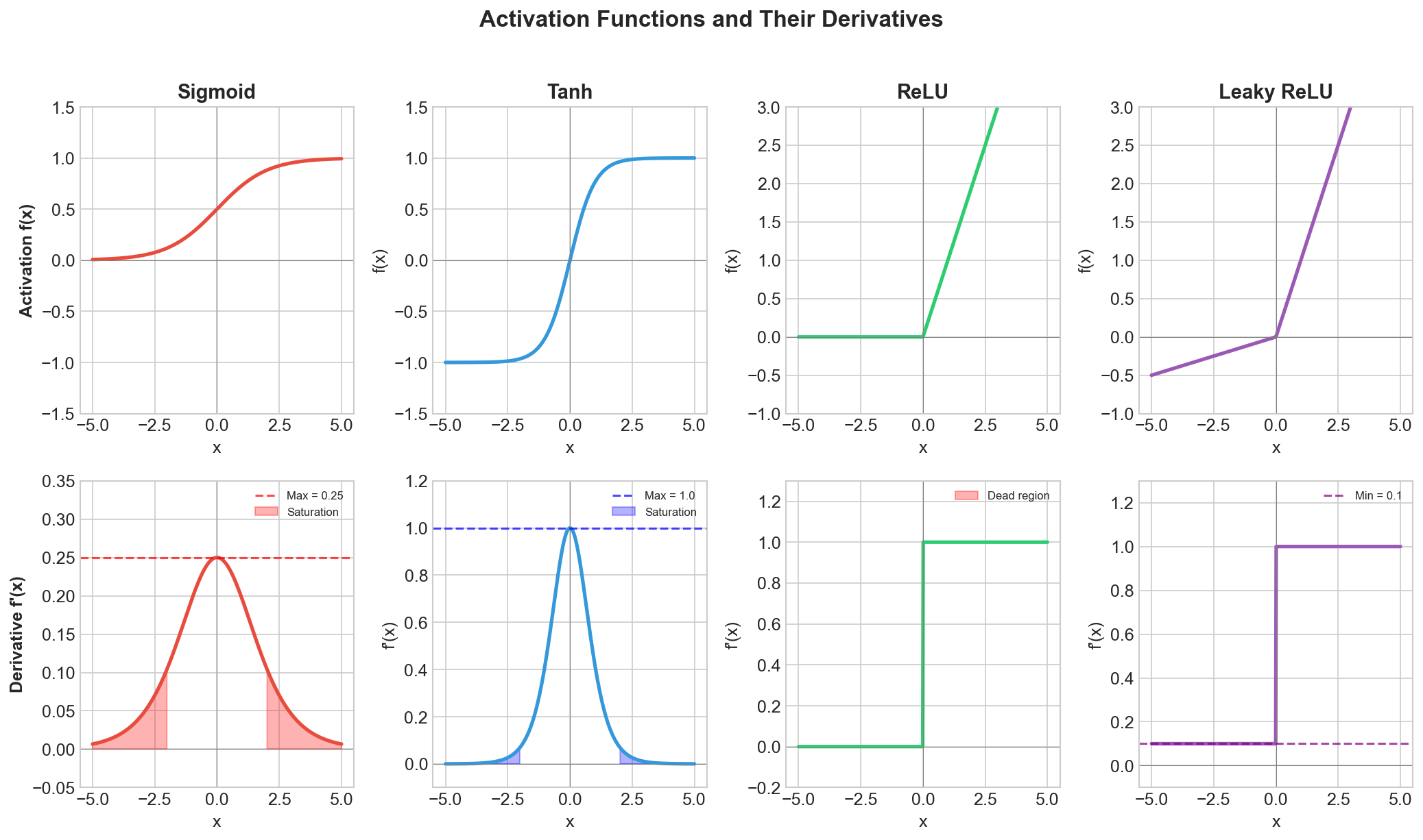
The visualization above shows how different activation functions behave and why their derivatives matter for gradient flow:

• Sigmoid: Max derivative 0.25, always shrinks gradients by 75%+
• Tanh: Max derivative 1.0 at x=0, but saturates for large inputs
• ReLU: Derivative is exactly 1 for positive inputs (no shrinking), but 0 for negative (dead neurons)
• Leaky ReLU: Never zero gradient, prevents dead neurons

Comparison Table:

Activation	Derivative Range	Vanishing Risk	Dead Neuron Risk
Sigmoid	(0, 0.25]	High	No
Tanh	(0, 1]	Medium	No
ReLU		Low	High
Leaky ReLU		Very Low	No
ELU	(0, 1]	Low	No
GELU	Smooth	Low	No

---

Q6: Why is ReLU preferred over sigmoid for hidden layers?

Answer: ReLU is preferred for several reasons:

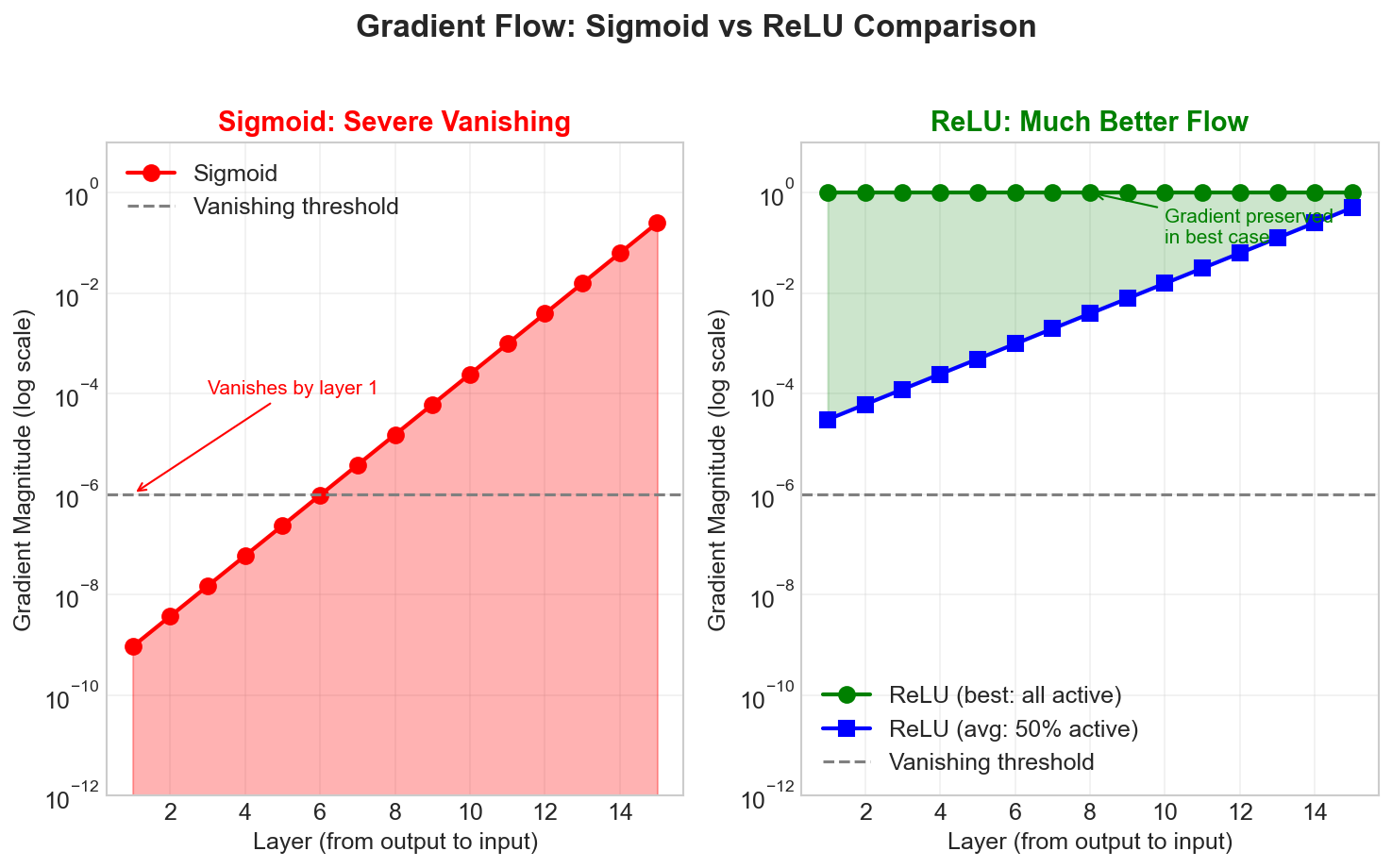
The visualization demonstrates why ReLU dramatically improves gradient flow:

Key Advantages:

1. No Gradient Saturation: Derivative is exactly 1 for positive inputs
2. Computational Efficiency: Simple threshold vs exponential computation
3. Sparse Activation: Zero for negative inputs creates beneficial sparsity

When to Still Use Sigmoid/Tanh:

• Output layer for binary classification (sigmoid)
• LSTM/GRU gates (sigmoid for gating, tanh for state)
• When bounded outputs are required

---

Q7: What is the dying ReLU problem and how do you fix it?

Answer: The dying ReLU problem occurs when neurons get stuck outputting zero for all inputs, effectively "dying" and never recovering.

Cause:

• If a neuron's weighted input is always negative
• Gradient is zero for negative inputs
• Weight never updates, neuron stays dead

Solutions:

1. Leaky ReLU:

def leaky_relu(x, alpha=0.01):
    return np.maximum(alpha * x, x)
    # Gradient is alpha (not 0) for negative inputs

2. Parametric ReLU (PReLU):

# Alpha is learnable
class PReLU(nn.Module):
    def __init__(self):
        super().__init__()
        self.alpha = nn.Parameter(torch.tensor(0.01))

    def forward(self, x):
        return torch.maximum(self.alpha * x, x)

3. ELU (Exponential Linear Unit):

def elu(x, alpha=1.0):
    return np.where(x > 0, x, alpha * (np.exp(x) - 1))
    # Smooth, non-zero gradient for negative inputs

4. GELU (Gaussian Error Linear Unit):

def gelu(x):
    return x * 0.5 * (1 + torch.erf(x / np.sqrt(2)))
    # Used in transformers (BERT, GPT)

5. Proper Initialization:

• He initialization helps prevent neurons from starting dead

---

Weight Initialization

Q8: What is Xavier/Glorot initialization and when should you use it?

Answer: Xavier (Glorot) initialization sets weights to maintain variance of activations across layers, preventing both vanishing and exploding gradients.

Formula:

W ~ Uniform(-sqrt(6/(n_in + n_out)), sqrt(6/(n_in + n_out)))
# or
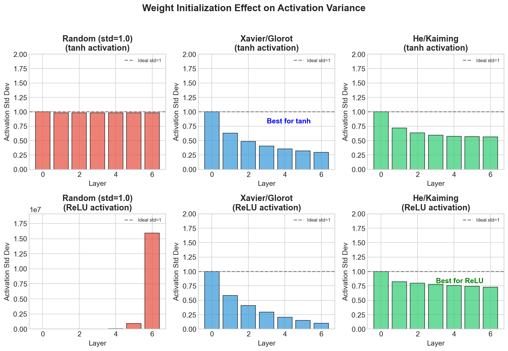
W ~ Normal(0, sqrt(2/(n_in + n_out)))

The visualization shows how Xavier maintains stable activation variance through layers with tanh activation, while random initialization causes issues.

Implementation:

import torch.nn as nn

# PyTorch built-in
nn.init.xavier_uniform_(layer.weight)
nn.init.xavier_normal_(layer.weight)

Use Xavier When: Using tanh or sigmoid activations, or symmetric activation functions.

---

Q9: What is He initialization and when should you use it?

Answer: He initialization is designed specifically for ReLU and its variants, accounting for the fact that ReLU zeros out half the inputs.

Formula:

W ~ Normal(0, sqrt(2/n_in))
# or
W ~ Uniform(-sqrt(6/n_in), sqrt(6/n_in))

Why Different from Xavier? ReLU sets ~50% of activations to zero, halving the variance. He compensates with a factor of 2.

As shown in the weight initialization visualization above, He initialization maintains stable activation variance through layers with ReLU, while Xavier causes gradual decay.

Implementation:

import torch.nn as nn

# PyTorch built-in
nn.init.kaiming_uniform_(layer.weight, nonlinearity='relu')
nn.init.kaiming_normal_(layer.weight, nonlinearity='relu')

Comparison:

Initialization	Formula (Variance)	Best For
Xavier	2/(n_in + n_out)	Tanh, Sigmoid
He	2/n_in	ReLU variants
LeCun	1/n_in	SELU

---

Q10: How do you initialize weights in practice for modern architectures?

Answer: Modern architectures often use specific initialization strategies:

Transformers:

# GPT-style initialization
def init_weights(module):
    if isinstance(module, nn.Linear):
        # Normal with small std
        nn.init.normal_(module.weight, mean=0.0, std=0.02)
        if module.bias is not None:
            nn.init.zeros_(module.bias)
    elif isinstance(module, nn.Embedding):
        nn.init.normal_(module.weight, mean=0.0, std=0.02)
    elif isinstance(module, nn.LayerNorm):
        nn.init.ones_(module.weight)
        nn.init.zeros_(module.bias)

ResNets:

# Zero-initialize last BN in each residual branch
# So residual blocks start as identity
for m in self.modules():
    if isinstance(m, Bottleneck):
        nn.init.zeros_(m.bn3.weight)

CNNs:

# He initialization for conv layers
for m in self.modules():
    if isinstance(m, nn.Conv2d):
        nn.init.kaiming_normal_(m.weight, mode='fan_out', nonlinearity='relu')

---

Normalization Techniques

Q11: How does batch normalization help with gradient flow?

Answer: Batch normalization addresses vanishing/exploding gradients by normalizing layer inputs, keeping activations in well-behaved ranges.

Mechanism:

def batch_norm(x, gamma, beta, eps=1e-5):
    # x shape: (batch_size, features)
    mean = x.mean(dim=0)
    var = x.var(dim=0)

    # Normalize to zero mean, unit variance
    x_norm = (x - mean) / torch.sqrt(var + eps)

    # Scale and shift (learnable)
    return gamma * x_norm + beta

Why It Helps:

1. Prevents Activation Saturation:

• Keeps inputs to activation functions near zero
• Sigmoid/tanh derivatives are largest near zero

2. Reduces Internal Covariate Shift:

• Each layer sees consistent input distribution
• Earlier layers don't have to adapt to changing distributions

3. Allows Higher Learning Rates:

• Normalized gradients are more stable
• Can use larger steps without exploding

4. Regularization Effect:

• Batch statistics add noise
• Acts as mild regularizer

Interview Follow-up - Gradient Through BatchNorm:

# Backprop through batch norm is non-trivial
# Gradient flows through both normalization and statistics
# This is why batch norm helps - it controls gradient magnitude

# Simplified gradient:
# ∂L/∂x ≈ γ/σ × (∂L/∂y - mean(∂L/∂y) - x_norm × mean(∂L/∂y × x_norm))

---

Q12: What is layer normalization and when is it preferred over batch norm?

Answer: Layer normalization normalizes across features instead of across the batch, making it suitable for RNNs and Transformers.

Key Difference:

# Batch Norm: normalize across batch dimension
# x shape: (batch, features)
x_bn = (x - x.mean(dim=0)) / x.std(dim=0)  # Statistics per feature

# Layer Norm: normalize across feature dimension
x_ln = (x - x.mean(dim=1, keepdim=True)) / x.std(dim=1, keepdim=True)  # Statistics per sample

When to Use Layer Norm:

1. Recurrent Neural Networks:

• Batch statistics don't make sense across time steps
• Each time step has different sequence positions

2. Transformers:

• Variable sequence lengths
• Layer norm is standard in BERT, GPT, etc.

3. Small Batch Sizes:

• Batch norm needs sufficient batch size for stable statistics
• Layer norm works with batch size = 1

4. Online/Streaming Inference:

• No batch available
• Layer norm computes per-sample

Transformer Usage:

class TransformerBlock(nn.Module):
    def __init__(self, d_model):
        super().__init__()
        self.attention = MultiHeadAttention(d_model)
        self.ffn = FeedForward(d_model)
        self.ln1 = nn.LayerNorm(d_model)
        self.ln2 = nn.LayerNorm(d_model)

    def forward(self, x):
        # Pre-norm architecture (GPT-2 style)
        x = x + self.attention(self.ln1(x))
        x = x + self.ffn(self.ln2(x))
        return x

---

Q13: Compare different normalization techniques.

Answer:

Technique	Normalizes Across	Use Case	Batch Dependent
Batch Norm	Batch dimension	CNNs, large batches	Yes
Layer Norm	Feature dimension	RNNs, Transformers	No
Instance Norm	Spatial dimensions	Style transfer	No
Group Norm	Channel groups	Small batch CNNs	No
RMS Norm	Feature dimension	LLMs (LLaMA)	No

Implementation Comparison:

import torch
import torch.nn as nn

x = torch.randn(32, 64, 28, 28)  # (batch, channels, height, width)

# Batch Norm - normalize per channel across batch & spatial
bn = nn.BatchNorm2d(64)
# Computes mean/var of shape (64,) across (32, 28, 28)

# Layer Norm - normalize across all features per sample
ln = nn.LayerNorm([64, 28, 28])
# Computes mean/var per sample across (64, 28, 28)

# Instance Norm - normalize per channel per sample
inn = nn.InstanceNorm2d(64)
# Computes mean/var of shape (32, 64) across (28, 28)

# Group Norm - normalize per group of channels
gn = nn.GroupNorm(num_groups=8, num_channels=64)
# Splits 64 channels into 8 groups of 8

RMS Norm (used in modern LLMs):

class RMSNorm(nn.Module):
    def __init__(self, dim, eps=1e-6):
        super().__init__()
        self.weight = nn.Parameter(torch.ones(dim))
        self.eps = eps

    def forward(self, x):
        # No mean subtraction, just RMS normalization
        rms = torch.sqrt(torch.mean(x**2, dim=-1, keepdim=True) + self.eps)
        return x / rms * self.weight

---

Architectural Solutions

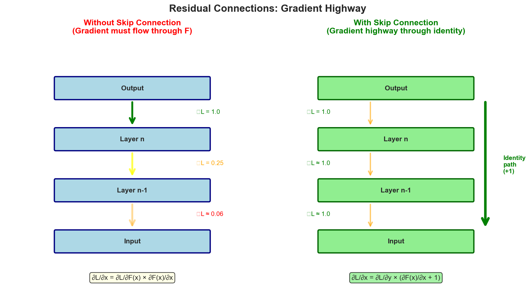
Q14: How do residual connections (skip connections) help with gradient flow?

Answer: Residual connections provide a direct path for gradients to flow backward, bypassing problematic layers.

Basic Residual Block:

class ResidualBlock(nn.Module):
    def __init__(self, channels):
        super().__init__()
        self.conv1 = nn.Conv2d(channels, channels, 3, padding=1)
        self.bn1 = nn.BatchNorm2d(channels)
        self.conv2 = nn.Conv2d(channels, channels, 3, padding=1)
        self.bn2 = nn.BatchNorm2d(channels)

    def forward(self, x):
        residual = x
        out = F.relu(self.bn1(self.conv1(x)))
        out = self.bn2(self.conv2(out))
        out = out + residual  # Skip connection
        return F.relu(out)

Why It Works - Gradient Analysis:

The diagram above illustrates the key insight. With skip connection (y = F(x) + x):

dL/dx = dL/dy * (dF(x)/dx + 1)

Even if dF(x)/dx approaches 0, gradient still flows through the +1 term via the identity path.

Benefits:

1. Gradient Highway: Direct path from loss to early layers
2. Identity Mapping: Easy to learn identity (set F(x) to 0)
3. Enables Very Deep Networks: ResNet-152, ResNet-1000 possible

---

Q15: How do LSTM gates specifically address vanishing gradients in RNNs?

Answer: LSTMs use a cell state with additive updates and gating mechanisms to maintain gradient flow across long sequences.

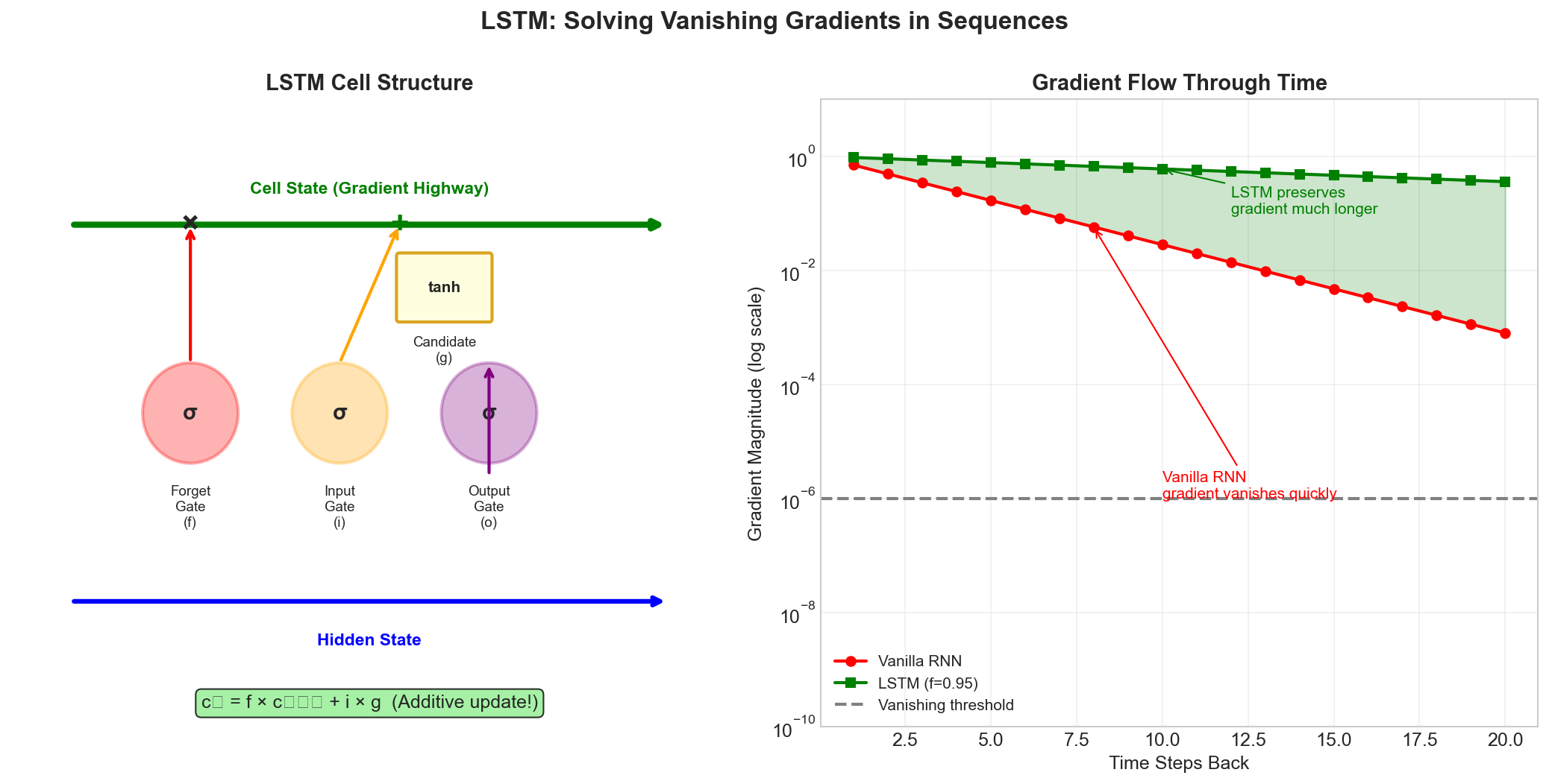
The Problem with Vanilla RNNs: Gradient through time involves a product of many weight matrices and tanh derivatives, causing exponential decay.

LSTM Solution - Cell State Highway:

class LSTMCell(nn.Module):
    def forward(self, x, hidden):
        h_prev, c_prev = hidden

        # Gate activations
        i = torch.sigmoid(...)  # Input gate
        f = torch.sigmoid(...)  # Forget gate (KEY!)
        g = torch.tanh(...)     # Candidate cell state
        o = torch.sigmoid(...)  # Output gate

        # Cell state update (KEY: additive, not multiplicative!)
        c_t = f * c_prev + i * g
        h_t = o * torch.tanh(c_t)

        return h_t, c_t

Why LSTM Works:

The visualization shows the key insight: the cell state acts as a "gradient highway."

1. Additive Update: c_t = f * c_{t-1} + i * g allows gradient to flow directly through addition
2. Forget Gate Near 1: When f is close to 1, gradient passes through unchanged
3. Gradient Path: dL/dc_0 = dL/dc_T * product(f_t) - product of forget gates can stay near 1

---

Q16: How does GRU compare to LSTM for gradient flow?

Answer: GRU (Gated Recurrent Unit) is a simplified version of LSTM with fewer parameters but similar gradient flow properties.

GRU Architecture:

class GRUCell(nn.Module):
    def __init__(self, input_size, hidden_size):
        super().__init__()
        self.hidden_size = hidden_size
        self.W_z = nn.Linear(input_size + hidden_size, hidden_size)  # Update gate
        self.W_r = nn.Linear(input_size + hidden_size, hidden_size)  # Reset gate
        self.W_h = nn.Linear(input_size + hidden_size, hidden_size)  # Candidate

    def forward(self, x, h_prev):
        combined = torch.cat([x, h_prev], dim=1)

        # Update gate (like LSTM forget gate)
        z = torch.sigmoid(self.W_z(combined))

        # Reset gate (controls h_prev contribution to candidate)
        r = torch.sigmoid(self.W_r(combined))

        # Candidate hidden state
        combined_reset = torch.cat([x, r * h_prev], dim=1)
        h_candidate = torch.tanh(self.W_h(combined_reset))

        # Final hidden state (interpolation)
        h_t = (1 - z) * h_prev + z * h_candidate

        return h_t

Comparison:

Aspect	LSTM	GRU
Gates	3 (input, forget, output)	2 (update, reset)
States	2 (hidden, cell)	1 (hidden)
Parameters	More	Fewer (~25% less)
Gradient Path	Through cell state	Through hidden state
Performance	Better on complex tasks	Better on smaller data

Gradient Flow in GRU:

h_t = (1-z) × h_{t-1} + z × h̃_t
∂h_t/∂h_{t-1} = (1-z) + z × ∂h̃_t/∂h_{t-1}

When z ≈ 0, gradient flows directly through (1-z) ≈ 1.

---

Gradient Clipping

Q17: What is gradient clipping and how do you implement it?

Answer: Gradient clipping limits gradient magnitudes to prevent exploding gradients, ensuring stable training.

Two Main Types:

1. Gradient Norm Clipping (Preferred):

# Clip by global norm
def clip_grad_norm(parameters, max_norm):
    total_norm = 0
    for p in parameters:
        if p.grad is not None:
            total_norm += p.grad.data.norm(2).item() ** 2
    total_norm = total_norm ** 0.5

    clip_coef = max_norm / (total_norm + 1e-6)
    if clip_coef < 1:
        for p in parameters:
            if p.grad is not None:
                p.grad.data.mul_(clip_coef)

    return total_norm

# PyTorch built-in
torch.nn.utils.clip_grad_norm_(model.parameters(), max_norm=1.0)

2. Gradient Value Clipping:

# Clip each gradient element independently
def clip_grad_value(parameters, clip_value):
    for p in parameters:
        if p.grad is not None:
            p.grad.data.clamp_(-clip_value, clip_value)

# PyTorch built-in
torch.nn.utils.clip_grad_value_(model.parameters(), clip_value=0.5)

Training Loop with Gradient Clipping:

optimizer = torch.optim.Adam(model.parameters(), lr=1e-4)

for batch in dataloader:
    optimizer.zero_grad()

    loss = model(batch)
    loss.backward()

    # Clip gradients before optimizer step
    grad_norm = torch.nn.utils.clip_grad_norm_(model.parameters(), max_norm=1.0)

    # Log gradient norm for monitoring
    if grad_norm > 1.0:
        print(f"Gradient clipped: {grad_norm:.2f} -> 1.0")

    optimizer.step()

Choosing Clip Value:

• Start with max_norm=1.0 (common default)
• Monitor gradient norms during training
• If frequently clipping, may indicate other issues
• Typical values: 0.5 to 5.0

---

Q18: When should you use gradient clipping?

Answer: Gradient clipping is essential in certain scenarios:

Always Use For:

1. RNNs/LSTMs/GRUs: Long sequences prone to gradient explosion
2. Transformers: Attention can cause gradient spikes
3. GANs: Unstable adversarial training
4. Reinforcement Learning: High variance gradients

Consider For:

1. Very deep networks
2. When using high learning rates
3. Fine-tuning with limited data
4. Mixed precision training

Example - Transformer Training:

# Standard practice for transformer training
class TransformerTrainer:
    def __init__(self, model, lr=1e-4, warmup_steps=4000, max_grad_norm=1.0):
        self.model = model
        self.optimizer = torch.optim.AdamW(model.parameters(), lr=lr)
        self.max_grad_norm = max_grad_norm

    def train_step(self, batch):
        self.optimizer.zero_grad()

        loss = self.model(**batch).loss
        loss.backward()

        # Essential for stable transformer training
        torch.nn.utils.clip_grad_norm_(
            self.model.parameters(),
            self.max_grad_norm
        )

        self.optimizer.step()
        return loss.item()

Warning Signs You Need Clipping:

• Loss suddenly becomes NaN
• Loss spikes dramatically
• Weights grow very large
• Training becomes unstable

---

Diagnosis and Debugging

Q19: How do you diagnose vanishing gradients in practice?

Answer: Several techniques help identify vanishing gradients:

1. Monitor Gradient Statistics:

def compute_gradient_stats(model):
    stats = {}
    for name, param in model.named_parameters():
        if param.grad is not None:
            grad = param.grad.data
            stats[name] = {
                'mean': grad.mean().item(),
                'std': grad.std().item(),
                'max': grad.max().item(),
                'min': grad.min().item(),
                'norm': grad.norm().item()
            }
    return stats

# During training
for epoch in range(num_epochs):
    for batch in dataloader:
        loss = model(batch)
        loss.backward()

        # Check gradient stats
        stats = compute_gradient_stats(model)

        # Early layers should have reasonable gradients
        for name, s in stats.items():
            if s['norm'] < 1e-7:
                print(f"WARNING: Vanishing gradient in {name}")

        optimizer.step()
        optimizer.zero_grad()

2. Visualize Gradient Flow:

import matplotlib.pyplot as plt

def plot_gradient_flow(named_parameters):
    ave_grads = []
    layers = []
    for name, param in named_parameters:
        if param.requires_grad and param.grad is not None:
            layers.append(name)
            ave_grads.append(param.grad.abs().mean().item())

    plt.figure(figsize=(12, 6))
    plt.bar(range(len(ave_grads)), ave_grads, alpha=0.7)
    plt.xticks(range(len(ave_grads)), layers, rotation=90)
    plt.xlabel("Layers")
    plt.ylabel("Average Gradient Magnitude")
    plt.title("Gradient Flow Through Network")
    plt.tight_layout()
    plt.show()

3. Check Weight Updates:

def monitor_weight_updates(model, optimizer):
    # Store weights before update
    old_weights = {n: p.data.clone() for n, p in model.named_parameters()}

    optimizer.step()

    # Compare with new weights
    for name, param in model.named_parameters():
        change = (param.data - old_weights[name]).norm().item()
        weight_norm = param.data.norm().item()
        relative_change = change / (weight_norm + 1e-8)

        if relative_change < 1e-8:
            print(f"WARNING: {name} barely updating (rel change: {relative_change:.2e})")

Symptoms of Vanishing Gradients:

• Gradient norms decrease exponentially toward input layers
• Early layer weights don't change
• Loss plateaus at high value
• Training accuracy doesn't improve

---

Q20: How do you diagnose exploding gradients?

Answer: Exploding gradients are usually easier to detect:

1. Monitor Gradient Norms:

def check_for_explosion(model, threshold=100):
    total_norm = 0
    for param in model.parameters():
        if param.grad is not None:
            total_norm += param.grad.data.norm(2).item() ** 2
    total_norm = total_norm ** 0.5

    if total_norm > threshold:
        print(f"EXPLODING GRADIENT: norm = {total_norm:.2e}")
        return True
    return False

2. Track Loss for NaN/Inf:

def safe_training_step(model, batch, optimizer):
    optimizer.zero_grad()
    loss = model(batch)

    # Check for NaN loss
    if torch.isnan(loss) or torch.isinf(loss):
        print("ERROR: Loss is NaN/Inf - likely exploding gradients")
        return None

    loss.backward()

    # Check for NaN gradients
    for name, param in model.named_parameters():
        if param.grad is not None:
            if torch.isnan(param.grad).any() or torch.isinf(param.grad).any():
                print(f"ERROR: NaN/Inf gradient in {name}")
                return None

    optimizer.step()
    return loss.item()

3. TensorBoard Logging:

from torch.utils.tensorboard import SummaryWriter

writer = SummaryWriter('runs/gradient_analysis')

def log_gradients(model, step):
    for name, param in model.named_parameters():
        if param.grad is not None:
            writer.add_histogram(f'gradients/{name}', param.grad, step)
            writer.add_scalar(f'gradient_norm/{name}', param.grad.norm(), step)

Symptoms of Exploding Gradients:

• Loss becomes NaN or Inf
• Loss oscillates wildly or increases
• Weight values become very large
• Gradient norms increase exponentially toward input
• Model outputs NaN predictions

---

Q21: What's your debugging checklist for gradient problems?

Answer: Here's a systematic debugging approach:

Step 1: Verify Data Pipeline

# Check for NaN/Inf in inputs
for batch in dataloader:
    assert not torch.isnan(batch['input']).any(), "NaN in inputs"
    assert not torch.isinf(batch['input']).any(), "Inf in inputs"
    break

Step 2: Test with Small Network

# Verify training works on tiny model
small_model = SimplifiedModel(num_layers=2)
# If this works, problem is depth-related

Step 3: Check Initialization

# Verify weights are properly initialized
for name, param in model.named_parameters():
    print(f"{name}: mean={param.mean():.4f}, std={param.std():.4f}")
    # Should see reasonable values, not all zeros or huge numbers

Step 4: Monitor Activations

# Hook to capture activations
activations = {}
def hook_fn(name):
    def hook(module, input, output):
        activations[name] = output.detach()
    return hook

for name, layer in model.named_modules():
    layer.register_forward_hook(hook_fn(name))

# After forward pass, check activations
for name, act in activations.items():
    if act.abs().mean() < 1e-6:
        print(f"Dead layer: {name}")
    if act.abs().max() > 1000:
        print(f"Exploding activation: {name}")

Step 5: Reduce Learning Rate

# If exploding, try much smaller LR
optimizer = torch.optim.Adam(model.parameters(), lr=1e-6)

Step 6: Add Gradient Clipping

torch.nn.utils.clip_grad_norm_(model.parameters(), max_norm=1.0)

Step 7: Try Normalization

# Add batch/layer norm to problematic layers

Step 8: Use Residual Connections

# Add skip connections if network is deep

---

Advanced Topics

Q22: How do transformers handle gradient flow differently?

Answer: Transformers use several mechanisms for stable gradient flow:

1. Pre-Layer Normalization:

class PreNormTransformerBlock(nn.Module):
    def forward(self, x):
        # Normalize before attention (not after)
        # Provides more stable gradients
        x = x + self.attention(self.ln1(x))
        x = x + self.ffn(self.ln2(x))
        return x

2. Scaled Dot-Product Attention:

def scaled_attention(Q, K, V):
    d_k = Q.size(-1)
    # Scale by sqrt(d_k) to prevent softmax saturation
    scores = torch.matmul(Q, K.transpose(-2, -1)) / math.sqrt(d_k)
    weights = F.softmax(scores, dim=-1)
    return torch.matmul(weights, V)

3. Residual Connections Throughout:

# Every sub-layer has residual connection
x = x + Attention(x)
x = x + FFN(x)

4. Careful Initialization:

# GPT-2 style: scale residual projections
# Prevents output variance from growing with depth
self.c_proj.weight.data *= 1 / math.sqrt(2 * num_layers)

5. Gradient Checkpointing for Memory:

# Trade compute for memory, doesn't affect gradient magnitude
from torch.utils.checkpoint import checkpoint

class CheckpointedTransformer(nn.Module):
    def forward(self, x):
        for block in self.blocks:
            x = checkpoint(block, x)
        return x

---

Q23: How does mixed precision training affect gradient flow?

Answer: Mixed precision training (FP16/BF16) requires special handling for gradients:

Potential Issues:

1. FP16 has limited range (~6e-5 to 65504)
2. Small gradients can underflow to zero
3. Large gradients can overflow to infinity

Solution: Loss Scaling

# Automatic Mixed Precision in PyTorch
from torch.cuda.amp import autocast, GradScaler

scaler = GradScaler()

for batch in dataloader:
    optimizer.zero_grad()

    # Forward pass in FP16
    with autocast():
        loss = model(batch)

    # Scale loss to prevent gradient underflow
    scaler.scale(loss).backward()

    # Unscale gradients and clip
    scaler.unscale_(optimizer)
    torch.nn.utils.clip_grad_norm_(model.parameters(), max_norm=1.0)

    # Update weights (handles inf/nan)
    scaler.step(optimizer)
    scaler.update()

How Loss Scaling Works:

1. Multiply loss by scale factor (e.g., 65536)
2. Backprop (gradients are also scaled)
3. Unscale gradients before optimizer step
4. If overflow detected, skip update and reduce scale
5. Gradually increase scale when stable

BFloat16 Advantage:

• Same exponent range as FP32
• Less precision but better range
• Often doesn't need loss scaling

---

Q24: Summarize all solutions to vanishing/exploding gradients.

Answer: Complete solution summary:

For Vanishing Gradients:

Solution	Implementation	Effectiveness
ReLU activation	Replace sigmoid/tanh in hidden layers	High
Proper initialization	Xavier for tanh, He for ReLU	High
Batch/Layer normalization	Add after linear/conv layers	Very High
Residual connections	Add skip connections	Very High
LSTM/GRU for RNNs	Replace vanilla RNN	Very High
Shorter networks	Reduce depth if possible	Medium
Highway networks	Learnable skip connections	High

For Exploding Gradients:

Solution	Implementation	Effectiveness
Gradient clipping	clip_grad_norm with max=1.0	Very High
Proper initialization	Avoid large initial weights	High
Lower learning rate	Reduce by 10x	Medium
Batch normalization	Stabilizes activations	High
Weight regularization	L2 penalty	Medium
Gradient scaling	For mixed precision	High

Modern Best Practices:

class ModernNetwork(nn.Module):
    def __init__(self, input_dim, hidden_dim, num_layers):
        super().__init__()

        # 1. Proper initialization will be applied
        self.layers = nn.ModuleList()

        for i in range(num_layers):
            self.layers.append(nn.Sequential(
                nn.Linear(hidden_dim, hidden_dim),
                nn.LayerNorm(hidden_dim),  # 2. Normalization
                nn.GELU(),  # 3. Good activation
            ))

        # 4. Apply proper initialization
        self.apply(self._init_weights)

    def _init_weights(self, module):
        if isinstance(module, nn.Linear):
            nn.init.kaiming_normal_(module.weight, nonlinearity='relu')
            if module.bias is not None:
                nn.init.zeros_(module.bias)

    def forward(self, x):
        for layer in self.layers:
            # 5. Residual connections
            x = x + layer(x)
        return x

# Training with gradient clipping
optimizer = torch.optim.AdamW(model.parameters(), lr=1e-4)
for batch in dataloader:
    loss = model(batch)
    loss.backward()
    # 6. Gradient clipping
    torch.nn.utils.clip_grad_norm_(model.parameters(), max_norm=1.0)
    optimizer.step()
    optimizer.zero_grad()

---

Quick Reference

Visual Summary:

The visualizations in this FAQ illustrate the key concepts:

• Gradient Decay: How gradients vanish/explode through layers
• Activation Functions: Why derivatives matter for gradient flow
• Sigmoid vs ReLU: Dramatic difference in gradient preservation
• Weight Initialization: Xavier for tanh, He for ReLU
• Skip Connections: The "identity path" that preserves gradients
• LSTM Gates: Cell state as a gradient highway

Interview Checklist:

1. Define the problems: Vanishing = gradients approach 0, Exploding = gradients approach infinity
2. Root cause: Chain rule multiplication through deep networks
3. Activation functions: ReLU > tanh > sigmoid for hidden layers
4. Initialization: He for ReLU, Xavier for tanh/sigmoid
5. Normalization: BatchNorm for CNNs, LayerNorm for Transformers/RNNs
6. Architecture: Skip connections enable very deep networks
7. RNNs: LSTM/GRU gates maintain gradient flow
8. Clipping: Essential for RNNs and Transformers
9. Diagnosis: Monitor gradient norms, check for NaN, visualize flow
10. Modern practice: Combine multiple solutions

One-Liner Answers:

• Vanishing gradients: Use ReLU, proper initialization, normalization, and skip connections.
• Exploding gradients: Use gradient clipping, lower learning rate, and normalization.
• Why LSTM? Additive cell state updates provide gradient highway.
• Why ResNet? Skip connections add +1 to gradient, preventing vanishing.
• Why BatchNorm? Keeps activations in non-saturated range.