MDP Foundations

The mathematical framework for RL — states, actions, rewards, and the Markov property

---

What is Reinforcement Learning?

Reinforcement Learning (RL) is a computational approach where an agent learns to make decisions by interacting with an environment. Unlike supervised learning, RL does not require labeled input/output pairs. Instead, the agent discovers optimal behavior through trial and error, guided by reward signals.

The Agent-Environment Loop

The fundamental RL interaction follows a cyclic pattern:

1. Agent observes the current state $s_t$
2. Agent selects an action $a_t$ based on its policy
3. Environment transitions to a new state $s_{t+1}$
4. Agent receives a reward $r_{t+1}$
5. Repeat

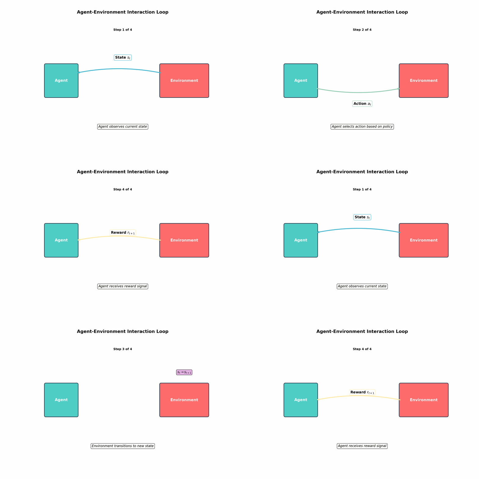
This loop captures the essence of sequential decision-making: every action influences future states and rewards, requiring the agent to balance immediate rewards against long-term consequences.

---

Markov Decision Process (MDP)

An MDP provides the formal mathematical framework for modeling RL problems. It defines the rules of the environment the agent interacts with.

Formal Definition

An MDP is defined by the tuple $(\mathcal{S},\mathcal{A},\mathcal{P},\mathcal{R},\gamma )$:

Component	Symbol	Description
State Space	$\mathcal{S}$	Set of all possible states the environment can be in
Action Space	$\mathcal{A}$	Set of all possible actions the agent can take
Transition Function	$\mathcal{P}(s^{\prime }\mid s,a)$	Probability of transitioning to state $s^{\prime }$ given state $s$ and action $a$
Reward Function	$\mathcal{R}(s,a,s^{\prime })$	Reward received for transition $(s,a,s^{\prime })$
Discount Factor	$\gamma \in [0,1]$	How much to weight future rewards vs. immediate rewards

Transition Dynamics

The transition function $\mathcal{P}:\mathcal{S}\times \mathcal{A}\times \mathcal{S}\to [0,1]$ defines the probability distribution over next states:

$$\mathcal{P}(s^{\prime }\mid s,a)=Pr(S_{t+1}=s^{\prime }\mid S_t=s,A_t=a)$$

This captures the stochastic nature of many environments — the same action in the same state may lead to different outcomes.

Reward Function Variants

The reward function can take several forms:

• $\mathcal{R}(s,a,s^{\prime })$: Reward depends on transition
• $\mathcal{R}(s,a)$: Reward depends on state-action pair
• $\mathcal{R}(s)$: Reward depends only on state

All forms are mathematically equivalent (can be converted to each other).

---

The Markov Property

The Markov property is the defining characteristic that makes MDPs tractable. It states:

$$Pr(S_{t+1}\mid S_t,A_t,S_{t-1},A_{t-1},\dots ,S_0,A_0)=Pr(S_{t+1}\mid S_t,A_t)$$

In plain terms: The future depends only on the current state, not on how we got there. The current state contains all relevant information for predicting what happens next.

Why the Markov Property Matters

Property	Implication
Memory-less	No need to store entire history
Computational tractability	Dynamic programming becomes possible
State sufficiency	State encodes everything needed for optimal decisions

When Markov Property Fails

Real-world problems often violate the Markov property:

• Partially Observable MDPs (POMDPs): Agent cannot fully observe the state
• History-dependent dynamics: Past actions affect future transitions

Solutions: Augment state with history, use recurrent neural networks, or model as POMDP.

---

Policies

A policy $\pi$ defines the agent's behavior — it specifies how the agent selects actions.

Deterministic Policies

A deterministic policy is a function mapping states to actions:

$$\pi :\mathcal{S}\to \mathcal{A}$$

Example: $\pi (s)=a$ means "always take action $a$ in state $s$"

Stochastic Policies

A stochastic policy defines a probability distribution over actions given a state:

$$\pi (a\mid s)=Pr(A_t=a\mid S_t=s)$$

Why stochastic?

• Exploration: Random actions help discover better strategies
• Game theory: Mixed strategies prevent exploitation by opponents
• Continuous action spaces: Often more natural representation

Policy Comparison

Type	Notation	Use Case
Deterministic	$\pi (s)=a$	Exploitation, optimal control
Stochastic	$\pi (a\mid s)$	Exploration, adversarial settings

---

Episodes vs. Continuing Tasks

RL problems fall into two categories based on their temporal structure.

Episodic Tasks

• Environment resets to initial state after reaching a terminal state
• Interaction naturally breaks into episodes
• Each episode is independent

Examples: Chess games, Atari games, robot manipulation tasks

Continuing Tasks

• No terminal states — interaction continues indefinitely
• Must handle infinite horizon
• Common in control and monitoring systems

Examples: Stock trading, power grid management, recommendation systems

Mathematical Difference

For episodic tasks, the return is:

$$G_t=R_{t+1}+R_{t+2}+\cdots +R_T$$

For continuing tasks, we must use discounting to ensure finite returns:

$$G_t=R_{t+1}+\gamma R_{t+2}+{\gamma }^2{R}_{t+3}+\cdots =\sum _{k=0}^{\mathrm{\infty }}{\gamma }^k{R}_{t+k+1}$$

---

Return and Discounted Return

The return $G_t$ quantifies the cumulative reward from time $t$ onward.

Discounted Return Formula

$$G_t=\sum _{k=0}^{\mathrm{\infty }}{\gamma }^k{R}_{t+k+1}=R_{t+1}+\gamma R_{t+2}+{\gamma }^2{R}_{t+3}+\cdots$$

Discount Factor $\gamma$

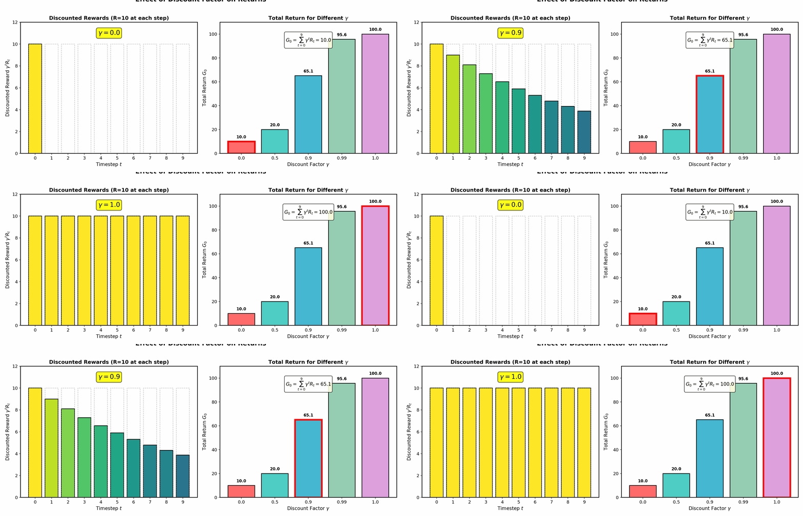
The discount factor $\gamma \in [0,1]$ controls the trade-off between immediate and future rewards:

$\gamma$ Value	Behavior
$\gamma =0$	Myopic: Only immediate reward matters
$\gamma \approx 0.5$	Balanced: Moderate future consideration
$\gamma \approx 0.99$	Far-sighted: Values future nearly as much as present
$\gamma =1$	No discounting: Only valid for episodic tasks

Why Discount?

1. Mathematical necessity: Ensures bounded returns for infinite-horizon problems
2. Uncertainty: Future is less predictable than present
3. Economic preference: Immediate rewards are often preferred (time value)
4. Convergence: Helps algorithms converge faster

Recursive Formulation

The return satisfies a useful recursive relationship:

$$G_t=R_{t+1}+\gamma G_{t+1}$$

This recursive structure is the foundation for dynamic programming methods like Bellman equations.

---

GridWorld Example

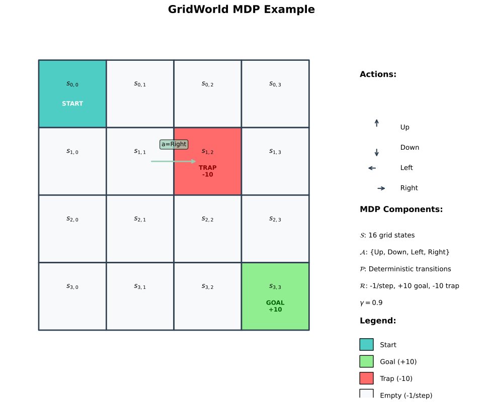
Consider a 4x4 grid where an agent navigates to a goal state:

Element	Description
States	16 grid cells $(0,0)$ to $(3,3)$
Actions	Up, Down, Left, Right
Transitions	Deterministic (walls cause stay in place)
Rewards	-1 per step, +10 at goal, -10 at trap
Discount	$\gamma =0.9$

The agent must learn to reach the goal while avoiding traps, minimizing steps taken.

---

Interview Questions

Q1: "Explain the Markov property and why it's important for RL."

The Markov property states that the future state depends only on the current state and action, not on the history of how we arrived at the current state:

$$Pr(S_{t+1}\mid S_t,A_t,S_{t-1},\dots ,S_0)=Pr(S_{t+1}\mid S_t,A_t)$$

Why it matters:

1. Computational tractability: We only need to track the current state, not the entire history
2. Enables dynamic programming: Bellman equations and value iteration rely on this property
3. State sufficiency: The optimal policy depends only on the current state

When it fails: In partially observable environments (POMDPs), the agent cannot see the full state. Solutions include maintaining belief states or using recurrent networks to encode history.

Q2: "What role does the discount factor play, and how do you choose it?"

The discount factor $\gamma \in [0,1]$ determines how much future rewards are weighted relative to immediate rewards:

$$G_t=R_{t+1}+\gamma R_{t+2}+{\gamma }^2{R}_{t+3}+\cdots$$

Key roles:

• Mathematical: Ensures convergence for infinite-horizon problems (geometric series)
• Behavioral: $\gamma \approx 0$ makes agent myopic; $\gamma \approx 1$ makes it far-sighted

Choosing $\gamma$:

• Episodic tasks: Often $\gamma =0.99$ or $1.0$
• Continuing tasks: Must be $<1$ for bounded returns
• Fast-changing environments: Lower $\gamma$ (e.g., 0.9) emphasizes near-term
• Long-term planning: Higher $\gamma$ (e.g., 0.999)

Practical tip: Start with $\gamma =0.99$, adjust based on task horizon.

Q3: "Compare deterministic vs. stochastic policies. When would you use each?"

Deterministic policy $\pi (s)=a$: Maps each state to exactly one action.

Stochastic policy $\pi (a\mid s)$: Defines a probability distribution over actions for each state.

Aspect	Deterministic	Stochastic
Exploration	No inherent exploration	Natural exploration via randomness
Optimality	Sufficient for most MDPs	Required for some POMDPs
Game theory	Exploitable	Mixed strategies can be optimal
Implementation	Simpler	More complex (sampling required)

Use deterministic when:

• Deploying a trained policy (exploitation)
• Full observability and no adversaries

Use stochastic when:

• Training (exploration is essential)
• Multi-agent or adversarial settings
• Partially observable environments

---

Quick Reference Card

MDP COMPONENTS
────────────────────────────────────────────────────────
S (States)        Set of environment configurations
A (Actions)       Set of agent choices
P(s'|s,a)         Transition probability function
R(s,a,s')         Reward function
γ (gamma)         Discount factor [0,1]

MARKOV PROPERTY
────────────────────────────────────────────────────────
P(S_{t+1}|S_t,A_t,...,S_0) = P(S_{t+1}|S_t,A_t)
Future depends only on current state, not history

POLICIES
────────────────────────────────────────────────────────
Deterministic:    π(s) = a
Stochastic:       π(a|s) = P(A=a|S=s)

RETURN
────────────────────────────────────────────────────────
Episodic:         G_t = Σ R_{t+k+1}
Discounted:       G_t = Σ γ^k R_{t+k+1}
Recursive:        G_t = R_{t+1} + γ G_{t+1}

DISCOUNT FACTOR γ
────────────────────────────────────────────────────────
γ = 0:            Myopic (only immediate reward)
γ = 0.9:          Standard starting point
γ = 0.99:         Far-sighted
γ = 1:            No discount (episodic only)

TASK TYPES
────────────────────────────────────────────────────────
Episodic:         Terminal states, finite episodes
Continuing:       No termination, infinite horizon

---

Key Takeaways

1. MDPs formalize sequential decision-making with states, actions, transitions, rewards, and discount factor.

2. The Markov property is foundational — it enables efficient algorithms by ensuring the current state contains all relevant information.

3. Discount factor $\gamma$ balances present vs. future — lower values emphasize immediate rewards, higher values encourage long-term planning.

4. Policies define agent behavior — deterministic for exploitation, stochastic for exploration and adversarial settings.

5. Understanding MDPs is prerequisite for value functions, Bellman equations, and all RL algorithms covered in subsequent modules.