Climbing Stairs & Knapsack Problems

Foundation DP problems with visualizations

---

Table of Contents

1. Climbing Stairs
2. 0/1 Knapsack Problem
3. Knapsack Variants
4. Interview Applications

---

Climbing Stairs

Problem Statement (LeetCode #70)

You are climbing a staircase. It takes n steps to reach the top. Each time you can either climb 1 or 2 steps. In how many distinct ways can you climb to the top?

Constraints:

• 1 <= n <= 45

Examples

Example 1: n = 2
Output: 2
Explanation: Two ways to climb:
  1. 1 step + 1 step
  2. 2 steps

Example 2: n = 3
Output: 3
Explanation: Three ways to climb:
  1. 1 step + 1 step + 1 step
  2. 1 step + 2 steps
  3. 2 steps + 1 step

Key Insight: Fibonacci Pattern

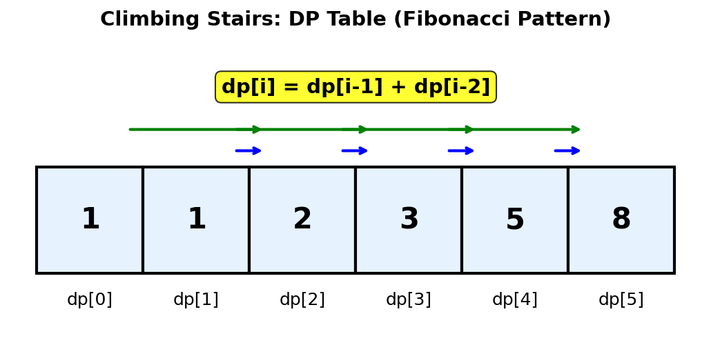
The climbing stairs problem exhibits optimal substructure - the number of ways to reach step n depends on the optimal solutions to subproblems for steps n-1 and n-2.

Recurrence Relation: dp[n] = dp[n-1] + dp[n-2]

Why? To reach step n, you can:
  - Come from step n-1 (take 1 step)
  - Come from step n-2 (take 2 steps)

DP State Visualization

Step:     0   1   2   3   4   5   6   7   8
         ─────────────────────────────────────
Ways:   [ 1 , 1 , 2 , 3 , 5 , 8 , 13, 21, 34 ]

                     Fibonacci sequence!

Visual Decision Tree for n=4:
                        ┌─────────┐
                        │  Step 4 │
                        │ dp[4]=5 │
                        └────┬────┘
               ┌─────────────┴─────────────┐
               │                           │
          ┌────┴────┐                 ┌────┴────┐
          │ Step 3  │                 │ Step 2  │
          │ dp[3]=3 │                 │ dp[2]=2 │
          └────┬────┘                 └────┬────┘
        ┌──────┴──────┐             ┌──────┴──────┐
   ┌────┴────┐  ┌────┴────┐   ┌────┴────┐  ┌────┴────┐
   │ Step 2  │  │ Step 1  │   │ Step 1  │  │ Step 0  │
   │ dp[2]=2 │  │ dp[1]=1 │   │ dp[1]=1 │  │ dp[0]=1 │
   └─────────┘  └─────────┘   └─────────┘  └─────────┘

Detailed breakdown for Step 5:
  ┌────────────────────────────────────────────────┐
  │ Step 5 can be reached from:                    │
  │                                                │
  │   From Step 4 (1 step) --> dp[4] = 5 ways     │
  │   From Step 3 (2 steps) --> dp[3] = 3 ways    │
  │                                                │
  │   Total: 5 + 3 = 8 ways                       │
  └────────────────────────────────────────────────┘

All Path Visualization for n=4

All 5 distinct paths to reach Step 4:

Path 1: 1 -> 1 -> 1 -> 1    (four 1-steps)
        ○ ─ ○ ─ ○ ─ ○ ─ ●
        0   1   2   3   4

Path 2: 1 -> 1 -> 2         (two 1-steps, one 2-step)
        ○ ─ ○ ─ ○ ═══ ●
        0   1   2     4

Path 3: 1 -> 2 -> 1         (1-step, 2-step, 1-step)
        ○ ─ ○ ═══ ○ ─ ●
        0   1     3   4

Path 4: 2 -> 1 -> 1         (2-step, two 1-steps)
        ○ ═══ ○ ─ ○ ─ ●
        0     2   3   4

Path 5: 2 -> 2              (two 2-steps)
        ○ ═══ ○ ═══ ●
        0     2     4

Legend: ─ = 1 step, ═══ = 2 steps

Solution Approaches

Approach 1: Naive Recursion (Don't use - exponential time)

def climbStairs_naive(n: int) -> int:
    """
    Time: O(2^n) - exponential!
    Space: O(n) - recursion stack
    """
    if n <= 2:
        return n
    return climbStairs_naive(n - 1) + climbStairs_naive(n - 2)

Complexity: Time O(2^n) · Space O(n)

• Time: Each call branches into two recursive calls, creating exponential tree
• Space: Maximum recursion depth is n for the call stack

Approach 2: Memoization (Top-Down DP)

def climbStairs_memo(n: int) -> int:
    """
    Time: O(n)
    Space: O(n)
    """
    memo = {}

    def dp(step):
        if step <= 2:
            return step
        if step in memo:
            return memo[step]

        memo[step] = dp(step - 1) + dp(step - 2)
        return memo[step]

    return dp(n)

Complexity: Time O(n) · Space O(n)

• Time: Each step computed exactly once due to memoization
• Space: Memo dictionary stores n values plus O(n) recursion stack

Approach 3: Tabulation (Bottom-Up DP)

def climbStairs_tabulation(n: int) -> int:
    """
    Time: O(n)
    Space: O(n)
    """
    if n <= 2:
        return n

    dp = [0] * (n + 1)
    dp[1] = 1
    dp[2] = 2

    for i in range(3, n + 1):
        dp[i] = dp[i - 1] + dp[i - 2]

    return dp[n]

Complexity: Time O(n) · Space O(n)

• Time: Single loop from 3 to n with O(1) work per iteration
• Space: DP array of size n+1 to store ways for each step

Approach 4: Space Optimized (Best Solution)

Python

def climbStairs(n: int) -> int:
    """
    Optimal Solution - Space O(1)

    Time: O(n)
    Space: O(1)
    """
    if n <= 2:
        return n

    # Only need the previous two values
    prev, curr = 1, 2

    for _ in range(3, n + 1):
        prev, curr = curr, prev + curr

    return curr

Java

public int climbStairs(int n) {
    if (n <= 2) return n;

    // Only need the previous two values
    int prev = 1, curr = 2;

    for (int i = 3; i <= n; i++) {
        int next = prev + curr;
        prev = curr;
        curr = next;
    }

    return curr;
}

Complexity: Time O(n) · Space O(1)

• Time: Single loop from 3 to n with O(1) work per iteration
• Space: Only two variables (prev, curr) instead of full array

Visual Guide

The following visualization shows the climbing stairs DP pattern, including the Fibonacci growth and golden ratio convergence:

Complexity Analysis

Approach	Time Complexity	Space Complexity
Naive Recursion	O(2^n)	O(n)
Memoization	O(n)	O(n)
Tabulation	O(n)	O(n)
Space Optimized	O(n)	O(1)
Matrix Exponentiation	O(log n)	O(1)

---

0/1 Knapsack Problem

Problem Statement

Given n items where each item has:

• weight[i]: The weight of item i
• value[i]: The value of item i

And a knapsack with maximum capacity W.

Goal: Find the maximum total value that can fit in the knapsack.

Constraint: Each item can only be taken once (0/1 choice - take it or leave it).

Why "0/1" Knapsack?

For each item, you have exactly 2 choices:
  - 0: Don't take the item
  - 1: Take the item (if it fits)

You CANNOT take a fraction of an item (unlike Fractional Knapsack).

DP State Definition

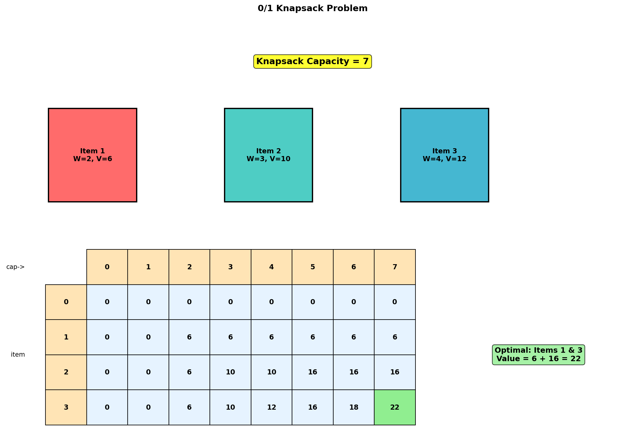
dp[i][w] = Maximum value achievable using first i items
           with knapsack capacity w

Recurrence:
  dp[i][w] = max(
      dp[i-1][w],                              # Don't take item i
      dp[i-1][w - weight[i]] + value[i]        # Take item i (if fits)
  )

Base case:
  dp[0][w] = 0  (no items = 0 value)
  dp[i][0] = 0  (no capacity = 0 value)

DP Table Visualization

Example:
  Items: weights = [1, 2, 3], values = [6, 10, 12]
  Capacity W = 5

Building the DP table step by step:

     Capacity -->
     0   1   2   3   4   5
   ┌───┬───┬───┬───┬───┬───┐
 0 │ 0 │ 0 │ 0 │ 0 │ 0 │ 0 │  No items available
   ├───┼───┼───┼───┼───┼───┤
 1 │ 0 │ 6 │ 6 │ 6 │ 6 │ 6 │  Item 1: w=1, v=6
   ├───┼───┼───┼───┼───┼───┤
 2 │ 0 │ 6 │10 │16 │16 │16 │  Item 2: w=2, v=10
   ├───┼───┼───┼───┼───┼───┤
 3 │ 0 │ 6 │10 │16 │18 │22 │  Item 3: w=3, v=12
   └───┴───┴───┴───┴───┴───┘
                         ↑
                    Answer: 22

Step-by-Step Table Construction

Row 1 (Item 1: w=1, v=6):
┌─────────────────────────────────────────────────────────────┐
│ For each capacity w from 0 to 5:                            │
│                                                             │
│ w=0: Can't fit item (w=1 > 0), dp[1][0] = 0                │
│ w=1: Can fit! max(dp[0][1], dp[0][0]+6) = max(0, 6) = 6    │
│ w=2: Can fit! max(dp[0][2], dp[0][1]+6) = max(0, 6) = 6    │
│ ...                                                         │
│ w=5: Can fit! max(dp[0][5], dp[0][4]+6) = max(0, 6) = 6    │
└─────────────────────────────────────────────────────────────┘

Row 2 (Item 2: w=2, v=10):
┌─────────────────────────────────────────────────────────────┐
│ w=0: dp[2][0] = 0                                           │
│ w=1: Can't fit (w=2 > 1), dp[2][1] = dp[1][1] = 6          │
│ w=2: Can fit! max(dp[1][2], dp[1][0]+10) = max(6, 10) = 10 │
│ w=3: Can fit! max(dp[1][3], dp[1][1]+10) = max(6, 16) = 16 │
│      (Take item 1 AND item 2: value = 6 + 10 = 16)         │
│ w=4: max(dp[1][4], dp[1][2]+10) = max(6, 16) = 16          │
│ w=5: max(dp[1][5], dp[1][3]+10) = max(6, 16) = 16          │
└─────────────────────────────────────────────────────────────┘

Row 3 (Item 3: w=3, v=12):
┌─────────────────────────────────────────────────────────────┐
│ w=3: max(dp[2][3], dp[2][0]+12) = max(16, 12) = 16         │
│      (Items 1+2 better than just item 3)                    │
│ w=4: max(dp[2][4], dp[2][1]+12) = max(16, 18) = 18         │
│      (Item 1 + Item 3: 6 + 12 = 18)                        │
│ w=5: max(dp[2][5], dp[2][2]+12) = max(16, 22) = 22         │
│      (Item 2 + Item 3: 10 + 12 = 22) <-- OPTIMAL!          │
└─────────────────────────────────────────────────────────────┘

Decision Path Visualization

Tracing back the optimal solution for dp[3][5] = 22:

Start at dp[3][5] = 22
  └── Is 22 > dp[2][5]=16? YES --> Item 3 was taken!
      Remaining capacity: 5 - 3 = 2
      Go to dp[2][2] = 10

At dp[2][2] = 10
  └── Is 10 > dp[1][2]=6? YES --> Item 2 was taken!
      Remaining capacity: 2 - 2 = 0
      Go to dp[1][0] = 0

At dp[1][0] = 0
  └── No more capacity, done!

Optimal selection:
┌─────────────────────────────────────────┐
│  Item 2 (w=2, v=10) +  ✓               │
│  Item 3 (w=3, v=12) +  ✓               │
│  ─────────────────────                  │
│  Total weight: 5                        │
│  Total value: 22                        │
└─────────────────────────────────────────┘

Solution Implementations

Approach 1: 2D DP Table (Standard)

def knapsack(weights: list[int], values: list[int], W: int) -> int:
    """
    Standard 0/1 Knapsack with 2D DP table

    Time: O(n * W)
    Space: O(n * W)
    """
    n = len(weights)

    # dp[i][w] = max value using first i items with capacity w
    dp = [[0] * (W + 1) for _ in range(n + 1)]

    for i in range(1, n + 1):
        for w in range(W + 1):
            # Option 1: Don't take item i
            dp[i][w] = dp[i-1][w]

            # Option 2: Take item i (if it fits)
            if weights[i-1] <= w:
                dp[i][w] = max(
                    dp[i][w],
                    dp[i-1][w - weights[i-1]] + values[i-1]
                )

    return dp[n][W]

Complexity: Time O(n * W) · Space O(n * W)

• Time: Nested loops iterate through n items and W capacity values
• Space: 2D DP table of size (n+1) x (W+1)

Approach 2: Space Optimized O(W)

Python

def knapsack_optimized(weights: list[int], values: list[int], W: int) -> int:
    """
    Space-optimized 0/1 Knapsack using 1D array

    Time: O(n * W)
    Space: O(W)

    Key insight: Each row only depends on the previous row.
    Traverse RIGHT TO LEFT to avoid using updated values.
    """
    dp = [0] * (W + 1)

    for i in range(len(weights)):
        # MUST traverse right to left!
        # This ensures we don't use an item multiple times
        for w in range(W, weights[i] - 1, -1):
            dp[w] = max(dp[w], dp[w - weights[i]] + values[i])

    return dp[W]


# Why right to left? Visualization:
"""
If we go left to right, we might use item i multiple times:

dp = [0, 0, 0, 0, 0, 0]  (W=5, item: w=2, v=10)

Left to right (WRONG for 0/1):
  w=2: dp[2] = max(0, dp[0]+10) = 10
  w=4: dp[4] = max(0, dp[2]+10) = 20  <-- Uses item twice!

Right to left (CORRECT):
  w=5: dp[5] = max(0, dp[3]+10) = 10
  w=4: dp[4] = max(0, dp[2]+10) = 10
  w=3: dp[3] = max(0, dp[1]+10) = 10
  w=2: dp[2] = max(0, dp[0]+10) = 10

Each item used at most once!
"""

Java

public int knapsackOptimized(int[] weights, int[] values, int W) {
    // Space-optimized 0/1 Knapsack using 1D array
    int[] dp = new int[W + 1];

    for (int i = 0; i < weights.length; i++) {
        // MUST traverse right to left to avoid using same item twice
        for (int w = W; w >= weights[i]; w--) {
            dp[w] = Math.max(dp[w], dp[w - weights[i]] + values[i]);
        }
    }

    return dp[W];
}

Complexity: Time O(n * W) · Space O(W)

• Time: Nested loops iterate through n items and W capacity values
• Space: Single 1D array of size W+1; right-to-left traversal prevents reusing items

Approach 3: With Item Reconstruction

def knapsack_with_items(weights: list[int], values: list[int], W: int) -> tuple[int, list[int]]:
    """
    Returns maximum value AND the items selected

    Time: O(n * W)
    Space: O(n * W)
    """
    n = len(weights)
    dp = [[0] * (W + 1) for _ in range(n + 1)]

    # Fill DP table
    for i in range(1, n + 1):
        for w in range(W + 1):
            dp[i][w] = dp[i-1][w]
            if weights[i-1] <= w:
                dp[i][w] = max(dp[i][w],
                              dp[i-1][w - weights[i-1]] + values[i-1])

    # Backtrack to find selected items
    selected_items = []
    w = W
    for i in range(n, 0, -1):
        if dp[i][w] != dp[i-1][w]:
            selected_items.append(i - 1)  # Item index (0-based)
            w -= weights[i - 1]

    selected_items.reverse()
    return dp[n][W], selected_items


# Example usage:
weights = [1, 2, 3]
values = [6, 10, 12]
W = 5

max_value, items = knapsack_with_items(weights, values, W)
print(f"Maximum value: {max_value}")  # 22
print(f"Selected items (indices): {items}")  # [1, 2] (items 2 and 3)

Complexity: Time O(n * W) · Space O(n * W)

• Time: O(n * W) for DP table plus O(n) for backtracking
• Space: Full 2D table required for backtracking to reconstruct selected items

Visual Guide

The following visualization shows the knapsack DP table as a heatmap with item selection:

Complexity Analysis

Approach	Time Complexity	Space Complexity
Brute Force	O(2^n)	O(n)
Memoization	O(n * W)	O(n * W)
2D Tabulation	O(n * W)	O(n * W)
1D Space Optimized	O(n * W)	O(W)

---

Knapsack Variants

1. Unbounded Knapsack

Each item can be used unlimited times.

def unbounded_knapsack(weights: list[int], values: list[int], W: int) -> int:
    """
    Unbounded Knapsack - items can be used multiple times

    Time: O(n * W)
    Space: O(W)

    Key difference: Traverse LEFT TO RIGHT (allow multiple uses)
    """
    dp = [0] * (W + 1)

    for w in range(1, W + 1):
        for i in range(len(weights)):
            if weights[i] <= w:
                dp[w] = max(dp[w], dp[w - weights[i]] + values[i])

    return dp[W]

Complexity: Time O(n * W) · Space O(W)

• Time: For each capacity, try all n items
• Space: Single 1D array of size W+1

# Alternative: Same as 0/1 but left-to-right inner loop
def unbounded_knapsack_v2(weights: list[int], values: list[int], W: int) -> int:
    dp = [0] * (W + 1)

    for i in range(len(weights)):
        # Left to right allows reusing item i
        for w in range(weights[i], W + 1):
            dp[w] = max(dp[w], dp[w - weights[i]] + values[i])

    return dp[W]

Complexity: Time O(n * W) · Space O(W)

• Time: Nested loops through n items and W capacity; left-to-right allows item reuse
• Space: Single 1D array of size W+1

2. Coin Change (Minimum Coins)

Given coins and amount, find minimum coins needed.

def coin_change(coins: list[int], amount: int) -> int:
    """
    LeetCode #322 - Coin Change
    Find minimum number of coins to make amount

    Time: O(n * amount)
    Space: O(amount)
    """
    dp = [float('inf')] * (amount + 1)
    dp[0] = 0  # 0 coins needed for amount 0

    for coin in coins:
        for a in range(coin, amount + 1):
            dp[a] = min(dp[a], dp[a - coin] + 1)

    return dp[amount] if dp[amount] != float('inf') else -1

Complexity: Time O(n * amount) · Space O(amount)

• Time: For each coin, iterate through all amounts from coin to target
• Space: Single 1D array of size amount+1

3. Coin Change II (Count Ways)

Count the number of combinations to make amount.

def coin_change_ways(coins: list[int], amount: int) -> int:
    """
    LeetCode #518 - Coin Change II
    Count number of ways to make amount

    Time: O(n * amount)
    Space: O(amount)
    """
    dp = [0] * (amount + 1)
    dp[0] = 1  # One way to make 0: use no coins

    for coin in coins:
        for a in range(coin, amount + 1):
            dp[a] += dp[a - coin]

    return dp[amount]

Complexity: Time O(n * amount) · Space O(amount)

• Time: Outer loop over coins, inner loop over amounts
• Space: Single 1D array of size amount+1

4. Subset Sum

Determine if a subset with given sum exists.

def subset_sum(nums: list[int], target: int) -> bool:
    """
    Can we form target sum using subset of nums?

    Time: O(n * target)
    Space: O(target)
    """
    dp = [False] * (target + 1)
    dp[0] = True  # Sum 0 always achievable (empty subset)

    for num in nums:
        # Right to left (0/1 - each element used once)
        for s in range(target, num - 1, -1):
            dp[s] = dp[s] or dp[s - num]

    return dp[target]

Complexity: Time O(n * target) · Space O(target)

• Time: For each number, iterate backwards through sums up to target
• Space: Boolean array of size target+1

5. Partition Equal Subset Sum

Can array be partitioned into two equal-sum subsets?

def can_partition(nums: list[int]) -> bool:
    """
    LeetCode #416 - Partition Equal Subset Sum

    Time: O(n * sum/2)
    Space: O(sum/2)
    """
    total = sum(nums)

    # Odd sum cannot be partitioned equally
    if total % 2 != 0:
        return False

    target = total // 2

    # Reduce to subset sum problem
    dp = [False] * (target + 1)
    dp[0] = True

    for num in nums:
        for s in range(target, num - 1, -1):
            dp[s] = dp[s] or dp[s - num]

    return dp[target]

Complexity: Time O(n * sum/2) · Space O(sum/2)

• Time: For each number, iterate backwards through sums up to sum/2
• Space: Boolean array of size target+1 where target = sum/2

Variant Comparison Table

┌──────────────────────────┬─────────────┬───────────────────────────┐
│ Variant                  │ Loop Order  │ Key Difference            │
├──────────────────────────┼─────────────┼───────────────────────────┤
│ 0/1 Knapsack            │ Right→Left  │ Each item used once       │
│ Unbounded Knapsack      │ Left→Right  │ Items can repeat          │
│ Coin Change (min coins) │ Left→Right  │ Minimize count            │
│ Coin Change II (ways)   │ Left→Right  │ Count combinations        │
│ Subset Sum              │ Right→Left  │ Boolean (exists or not)   │
│ Partition Equal Subset  │ Right→Left  │ Find if sum/2 achievable  │
└──────────────────────────┴─────────────┴───────────────────────────┘

---

Interview Applications

Common Interview Patterns

These fundamental DP problems are frequently tested at top tech companies. Here are real-world applications:

1. Resource Allocation

Scenario: Allocate servers to maximize throughput
- Each server type has different capacity (weight) and performance (value)
- Total budget constraint (knapsack capacity)
- Solution: 0/1 Knapsack if servers are unique, Unbounded if repeatable

2. Task Scheduling

Scenario: Complete tasks within time limit
- Each task has duration and reward
- Maximize reward within deadline
- Variation: Weighted Job Scheduling (DP with binary search)

3. Network Packet Optimization

Scenario: Select packets to transmit in limited bandwidth
- Packets have size and priority
- Maximize total priority within bandwidth
- Classic knapsack application

Related LeetCode Problems

Problem	Number	Difficulty	Pattern
Climbing Stairs	#70	Easy	Fibonacci DP
Min Cost Climbing Stairs	#746	Easy	Min-cost DP
House Robber	#198	Medium	Linear DP
Coin Change	#322	Medium	Unbounded Knapsack
Coin Change II	#518	Medium	Counting DP
Partition Equal Subset Sum	#416	Medium	Subset Sum
Target Sum	#494	Medium	Subset Sum variant
Last Stone Weight II	#1049	Medium	Knapsack variant
Ones and Zeroes	#474	Medium	2D Knapsack
Profitable Schemes	#879	Hard	3D Knapsack

Interview Tips

1. Identify the pattern first: Is it 0/1, unbounded, or subset sum?
2. Start with recurrence relation: Define dp[i] or dp[i][j] clearly
3. Consider space optimization: Interviewers often ask for O(W) or O(target) space
4. Practice reconstruction: Know how to trace back the actual items selected
5. Handle edge cases: Empty inputs, zero capacity, all items too heavy

---

Quick Reference

Climbing Stairs Formula

dp[i] = dp[i-1] + dp[i-2]
# Base: dp[0] = dp[1] = 1

0/1 Knapsack Formula

dp[i][w] = max(dp[i-1][w], dp[i-1][w-weight[i]] + value[i])
# Space optimized: traverse right to left

When to Use Each Pattern

Problem Type	Pattern	Loop Direction
Each item once	0/1 Knapsack	Right to Left
Items unlimited	Unbounded	Left to Right
Count combinations	Coin Change II	Left to Right
Check existence	Subset Sum	Right to Left
Fibonacci-like	Climbing Stairs	Forward

---

Prime Numbers & Sieve of Eratosthenes

Overview

While not a traditional DP problem, the Sieve of Eratosthenes shares similar characteristics with DP - it builds a solution incrementally using previously computed results. This algorithm is the most efficient way to find all prime numbers up to a given limit and appears frequently in coding interviews.

Problem Statement (LeetCode 204: Count Primes)

Given an integer n, return the number of prime numbers that are strictly less than n.

Examples:

Input: n = 10
Output: 4
Explanation: Primes less than 10 are [2, 3, 5, 7]

Input: n = 0 or n = 1
Output: 0
Explanation: No primes less than 0 or 1

Input: n = 2
Output: 0
Explanation: No primes strictly less than 2

What is a Prime Number?

A prime number is a natural number greater than 1 that has no positive divisors other than 1 and itself.

First few primes: 2, 3, 5, 7, 11, 13, 17, 19, 23, 29, ...

Key insight: 2 is the only even prime number

Naive Approach (Don't Use in Interviews)

def is_prime_naive(n: int) -> bool:
    """Check if n is prime - O(n) per number"""
    if n < 2:
        return False
    for i in range(2, n):
        if n % i == 0:
            return False
    return True


def count_primes_naive(n: int) -> int:
    """
    Count primes less than n.

    Time: O(n^2) - checking each number up to n
    Space: O(1)

    TOO SLOW for large n!
    """
    count = 0
    for i in range(2, n):
        if is_prime_naive(i):
            count += 1
    return count

Complexity: Time O(n^2) · Space O(1)

• Time: For each of n numbers, check up to n divisors
• Space: No additional data structures needed

Better: Check Up to Square Root

def is_prime_sqrt(n: int) -> bool:
    """
    Check if n is prime - O(sqrt(n)) per number.

    Key insight: If n = a * b, then min(a, b) <= sqrt(n).
    So we only need to check divisors up to sqrt(n).
    """
    if n < 2:
        return False
    if n == 2:
        return True
    if n % 2 == 0:
        return False

    for i in range(3, int(n ** 0.5) + 1, 2):
        if n % i == 0:
            return False
    return True


def count_primes_sqrt(n: int) -> int:
    """
    Time: O(n * sqrt(n))
    Space: O(1)

    Better, but still not optimal for large n.
    """
    count = 0
    for i in range(2, n):
        if is_prime_sqrt(i):
            count += 1
    return count

Complexity: Time O(n * sqrt(n)) · Space O(1)

• Time: For each of n numbers, check up to sqrt(n) divisors
• Space: No additional data structures needed

Optimal: Sieve of Eratosthenes

The Sieve of Eratosthenes is an ancient algorithm (circa 240 BC) that finds all primes up to n by iteratively marking multiples of each prime as composite.

Algorithm:

1. Create a boolean array is_prime[0..n-1], initialize all to True
2. Mark is_prime[0] and is_prime[1] as False (not prime)
3. For each number i from 2 to sqrt(n):
   • If is_prime[i] is True, mark all multiples of i as False
4. All remaining True values are primes

Visual Walkthrough

Sieve of Eratosthenes for n = 30:

Initial (all True except 0, 1):
Index:  0  1  2  3  4  5  6  7  8  9 10 11 12 13 14 15 16 17 18 19 20 21 22 23 24 25 26 27 28 29
        F  F  T  T  T  T  T  T  T  T  T  T  T  T  T  T  T  T  T  T  T  T  T  T  T  T  T  T  T  T

After marking multiples of 2:
        F  F  T  T  F  T  F  T  F  T  F  T  F  T  F  T  F  T  F  T  F  T  F  T  F  T  F  T  F  T
                    X     X     X     X     X     X     X     X     X     X     X     X     X     X

After marking multiples of 3:
        F  F  T  T  F  T  F  T  F  F  F  T  F  T  F  F  F  T  F  T  F  F  F  T  F  T  F  F  F  T
                                   X        X        X        X        X        X        X

After marking multiples of 5:
        F  F  T  T  F  T  F  T  F  F  F  T  F  T  F  F  F  T  F  T  F  F  F  T  F  F  F  F  F  T
                                                                                   X

sqrt(30) ≈ 5.47, so we're done!

Remaining primes: 2, 3, 5, 7, 11, 13, 17, 19, 23, 29 (10 primes < 30)

Solution

Python

def countPrimes(n: int) -> int:
    """
    Count primes less than n using Sieve of Eratosthenes.

    Time: O(n log log n) - nearly linear
    Space: O(n) for the sieve array

    Args:
        n: Upper limit (exclusive)

    Returns:
        Count of primes strictly less than n
    """
    if n <= 2:
        return 0

    # Initialize sieve: True means potentially prime
    is_prime = [True] * n
    is_prime[0] = is_prime[1] = False

    # Only need to sieve up to sqrt(n)
    for i in range(2, int(n ** 0.5) + 1):
        if is_prime[i]:
            # Mark all multiples of i as composite
            # Start from i*i because smaller multiples already marked
            for j in range(i * i, n, i):
                is_prime[j] = False

    return sum(is_prime)


def sieve_of_eratosthenes(n: int) -> list[int]:
    """
    Return list of all primes less than n.

    Time: O(n log log n)
    Space: O(n)
    """
    if n <= 2:
        return []

    is_prime = [True] * n
    is_prime[0] = is_prime[1] = False

    for i in range(2, int(n ** 0.5) + 1):
        if is_prime[i]:
            for j in range(i * i, n, i):
                is_prime[j] = False

    return [i for i in range(n) if is_prime[i]]

Java

public int countPrimes(int n) {
    if (n <= 2) return 0;

    // Initialize sieve: true means potentially prime
    boolean[] isPrime = new boolean[n];
    Arrays.fill(isPrime, true);
    isPrime[0] = isPrime[1] = false;

    // Only need to sieve up to sqrt(n)
    for (int i = 2; (long) i * i < n; i++) {
        if (isPrime[i]) {
            // Mark all multiples of i as composite
            // Start from i*i because smaller multiples already marked
            for (int j = i * i; j < n; j += i) {
                isPrime[j] = false;
            }
        }
    }

    int count = 0;
    for (boolean p : isPrime) if (p) count++;
    return count;
}

Complexity: Time O(n log log n) · Space O(n)

• Time: Inner loop iterations sum to n * (1/2 + 1/3 + 1/5 + ...) = n log log n
• Space: Boolean sieve array of size n

Optimized Version (Skip Even Numbers)

def countPrimes_optimized(n: int) -> int:
    """
    Optimized sieve that handles 2 separately and only sieves odd numbers.

    Time: O(n log log n)
    Space: O(n/2) ≈ O(n)

    Approximately 2x faster and uses half the memory.
    """
    if n <= 2:
        return 0
    if n == 3:
        return 1

    # Only store odd numbers: is_prime[i] represents 2*i + 1
    # e.g., is_prime[0] = False (represents 1)
    #       is_prime[1] = True  (represents 3)
    #       is_prime[2] = True  (represents 5)
    size = (n - 1) // 2
    is_prime = [True] * size
    is_prime[0] = False  # 1 is not prime

    # Sieve odd numbers starting from 3
    limit = int(n ** 0.5)
    for i in range(1, (limit + 1) // 2):
        if is_prime[i]:
            # i represents the number 2*i + 1
            p = 2 * i + 1
            # Mark multiples of p, starting from p*p
            # p*p in our indexing: (p*p - 1) // 2
            start = (p * p - 1) // 2
            for j in range(start, size, p):
                is_prime[j] = False

    # Count: 1 for the number 2, plus all True values
    return 1 + sum(is_prime)

Complexity: Time O(n log log n) · Space O(n/2)

• Time: Same asymptotic complexity, but ~2x faster in practice by skipping evens
• Space: Half the memory since only odd numbers are stored

Complexity Analysis

Approach	Time Complexity	Space Complexity
Naive (check all divisors)	O(n^2)	O(1)
Square root check	O(n * sqrt(n))	O(1)
Sieve of Eratosthenes	O(n log log n)	O(n)
Optimized Sieve (odd only)	O(n log log n)	O(n/2)

Why O(n log log n)?

The inner loop runs approximately n/2 + n/3 + n/5 + n/7 + ... times (once for each prime). This sum equals n * (1/2 + 1/3 + 1/5 + 1/7 + ...) = n * log(log(n)) by the Prime Harmonic Series.

Mermaid Diagram: Sieve Process

Related Problems

Problem	Difficulty	Key Concept
Count Primes (LC 204)	Medium	Sieve of Eratosthenes
Prime Number of Set Bits (LC 762)	Easy	Prime check + bit counting
Ugly Number (LC 263)	Easy	Prime factorization
Ugly Number II (LC 264)	Medium	DP with prime factors
Four Divisors (LC 1390)	Medium	Prime factorization

Interview Tips

1. Know the naive approach first: Explain the O(sqrt(n)) check before jumping to the sieve
2. Explain the optimization: Start from ii, not i2, because smaller multiples were already marked
3. Handle edge cases: n <= 2 returns 0 (no primes less than 2)
4. Memory trade-off: Sieve uses O(n) space but is much faster than O(1) space approaches
5. Segmented Sieve: For very large n that doesn't fit in memory, mention the segmented sieve variant

Why This Appears in DP Sections

The sieve shares key characteristics with DP:

• Builds incrementally: Each step uses results from previous steps
• Memoization: We store computed results (is_prime array)
• Subproblem dependency: Marking multiples depends on knowing primes found so far

---

Sources

• Climbing Stairs - LeetCode
• 70. Climbing Stairs - In-Depth Explanation
• Climbing stairs to reach the top - GeeksforGeeks
• 0/1 Knapsack Problem - GeeksforGeeks
• DSA The 0/1 Knapsack Problem - W3Schools
• Demystifying the 0-1 knapsack problem - Educative
• How to solve the Knapsack Problem with dynamic programming - Medium